
Inside the Model: Interpretability · Part 10 of 12
What Training Builds Inside a Model, Snapshot by Snapshot
Word counts, then word pairs, then induction heads in 300 steps: 49 snapshots of the From Scratch model show what forms when, and what set the timing.
On this page
TL;DR
A language model doesn’t learn everything at once. This part opens the 49 saved snapshots of the series’ own 88M-parameter model from From Scratch Part 7 and measures what is inside each one. The model first matches plain word frequencies (closest at step 50), then word pairs (closest at step 150), and then abandons both. Previous-token heads grow from step 50, and between steps 300 and 600 induction heads switch on: the best head’s score jumps from 0.03 to 0.63, the loss on a repeated random sequence falls from 11.8 to 6.7 nats, in-context learning appears, and the loss curve shows a small bump. Knocking out three heads at step 600 removes about 80% of that in-context learning. Seven smaller From Scratch runs and Pythia-70m built their induction heads between steps 250 and 1,000 too, though by then they had read anywhere from 33 million to 2 billion tokens.
Why it matters
At step 300 of its training run, the From Scratch model had read 157 million tokens and cut its validation loss from 9.8 to 4.65 nats, and it still couldn’t copy. Shown 50 random tokens and then the same 50 again, it predicted the second copy no better than the first: 11.8 nats per token on both. Three hundred steps later, with the same data and a smoothly decaying learning rate, it predicted the second copy at 6.7 nats, and by the end of training at 3.0.
Part 4 found the circuit that does this copying, the induction head, in finished models, and quoted Olsson et al.’s claim that these heads appear abruptly, together with a bump in the training loss. Part 7’s loss curve showed no visible bump. A finished model can’t say when or in what order its parts formed; a run that saved its weights along the way can.
The intuition
Think of a time-lapse of a building going up. A photo of the finished building tells you what’s there; the time-lapse tells you the order, foundations, then scaffolding, then the floors that need the scaffolding, and when each appeared.
Training snapshots are that time-lapse, and the loss curve is the calendar. The parts are what you can measure inside a snapshot: how close its predictions are to simple word statistics, where its attention heads look, what a probe can read from its vectors.
The analogy breaks in one place. Builders don’t tear down the foundations. A model does: the word-frequency predictions it fits early on get worse later, because something better replaces them.
Step 1: 49 snapshots and a way to look inside them
The model is From Scratch’s main run: 88 million parameters, 10 layers, 12 query heads per layer sharing 4 key-value heads (grouped-query attention), rotary position embeddings (RoPE), RMSNorm and a SwiGLU feed-forward layer (MLP) (written in From Scratch Part 4). It trained on 1.76 billion FineWeb-Edu tokens in 3,360 optimizer steps, weight updates, of 524,288 tokens each. The run saved 49 weights-only snapshots: the untrained weights, 14 extra ones in the first 250 steps (5, 10, 15, 20, 25, 30, 40, 50, 60, 75, 90, 125, 150, 250), one every 100 steps and the final step, 3,360. A snapshot named step N holds the weights after N updates.
The model computes attention with PyTorch’s fused scaled_dot_product_attention, which never writes the attention weights to memory, so there’s no pattern to read. Instead, a hook (a function PyTorch calls during the forward pass) saves each block’s attention input, and the new module lab/dynamics.py recomputes the pattern from it:
import math

import torch
import torch.nn.functional as F
from model import apply_rope   # From Scratch Part 4's RoPE (fromscratch/ on the path)


def attention_pattern(model, layer, x):
    """[B, n_head, T, T] attention weights of one block, recomputed in FP32 from its input x."""
    attn, cfg = model.blocks[layer].attn, model.cfg
    B, T, _ = x.shape
    x = x.float()
    q = F.linear(x, attn.wq.weight.float()).view(B, T, cfg.n_head, cfg.head_dim).transpose(1, 2)
    k = F.linear(x, attn.wk.weight.float()).view(B, T, cfg.n_kv_head, cfg.head_dim).transpose(1, 2)
    q, k = apply_rope(q, model.rope_cos, model.rope_sin), apply_rope(k, model.rope_cos, model.rope_sin)
    k = k.repeat_interleave(cfg.n_head // cfg.n_kv_head, dim=1)        # GQA: head h reads kv head h // 3
    s = (q @ k.transpose(-1, -2)) / math.sqrt(cfg.head_dim)
    mask = torch.ones(T, T, dtype=torch.bool, device=x.device).triu(1)
    return s.masked_fill(mask, float("-inf")).softmax(-1)
Queries and keys get RoPE, the rotation that encodes position, and each group of three query heads shares one key head, as in the model. Multiplying the recomputed pattern by the values reproduces the model’s own attention output to within 3 × 10⁻⁶ in FP32 (32-bit floats), in all 10 layers. The head scores come from Part 4’s lab/heads.py. Run from the folder that holds lab/:
from lab import dynamics as D

for step in (300, 600, 3360):
    model = D.load(f"{D.RUNS['main88'].path}/model_{step:05d}.pt", D.RUNS["main88"].cfg)  # FP32
    tok = D.repeated_tokens(200, 50, seed=1, allowed=D.frequent_tokens())              # [EOT] + r + r
    s = D.head_scores(model, tok, half=50)              # Part 4's scores for all 120 heads
    ind = s["induction"].mean(0)                         # [layer, head]
    l, h = divmod(int(ind.argmax()), ind.shape[1])
    print(f"step {step}: pattern check {D.check_patterns(model, tok[:8]):.0e}, "
          f"best induction head {l}.{h} ({ind.max():.2f}), "
          f"loss first copy {s['loss'][:, 1:50].mean():.1f}, second copy {s['loss'][:, 51:].mean():.1f}")
step 300: pattern check 2e-06, best induction head 8.10 (0.03), loss first copy 11.9, second copy 11.8
step 600: pattern check 2e-06, best induction head 8.10 (0.63), loss first copy 12.4, second copy 6.7
step 3360: pattern check 3e-06, best induction head 8.9 (0.84), loss first copy 11.8, second copy 3.0Heads are written layer.head, counting from 0. Every snapshot gets the same fixed measurements, all on an NVIDIA GeForce RTX 4060 Laptop GPU (8 GB) with PyTorch 2.11, plain hooks and no TransformerLens:
| Measurement | Data | Size |
|---|---|---|
| Induction and duplicate-token scores, copying loss | the end-of-text token, then 50 random tokens twice, drawn from the 9,875 tokens seen at least 1,000 times in the first 100 million training tokens | 200 sequences |
| Previous-token score | 256-token windows of held-out documents | 200 windows |
| In-context learning score | the first 512 tokens of held-out documents | 1,000 documents |
| Distance from word statistics | token counts over the first 100 million training tokens; held-out text | 32,704 positions |
The held-out text is the From Scratch validation shard, 15 million FineWeb-Edu tokens (ODC-By license) the model never trained on. The end-of-text token, which preceded every training document, serves as a start token. Scores run in FP32, losses on long windows under BF16 (16-bit) autocast, as in training.
Step 2: first word counts, then word pairs
The crudest model of text predicts each token from its overall frequency and ignores the context: a unigram model. One step up, a bigram model predicts from the current token alone, using how often each token follows it. Both come straight from counting, here over the first 100 million training tokens: 32,687 token types and 9,668,948 distinct pairs.
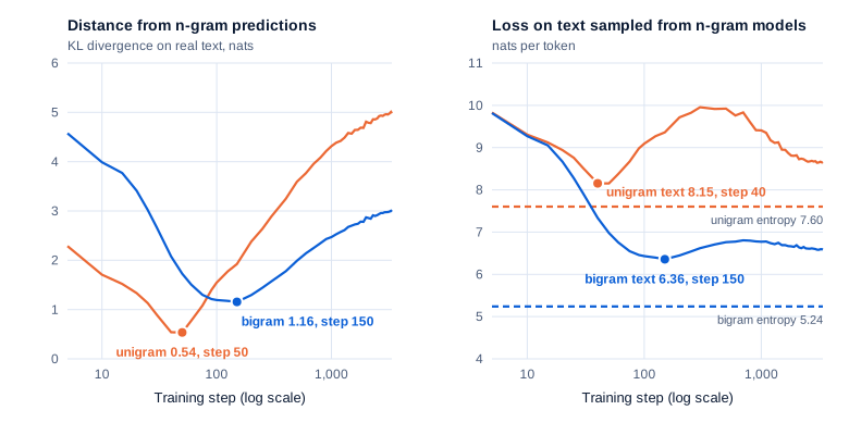
KL (Kullback-Leibler) divergence measures how far the model’s predicted distribution is from the n-gram model’s, in nats; 0 means identical. Belrose et al. (2024) measured it on Pythia checkpoints and argued for a distributional simplicity bias: networks learn the low-order statistics of their data first. Their sharper test scores the model on text sampled from the n-gram models themselves, which has those statistics and nothing else. Both ran on every snapshot here:
Swipe to pan the diagram, or tap it to zoom.
The unigram fit is best at step 50 and the bigram fit at step 150, both before any induction head exists.
| Step | Tokens seen | KL from unigram | KL from bigram | Loss on unigram text | Loss on bigram text | Validation loss |
|---|---|---|---|---|---|---|
| 5 | 2.6M | 2.29 | 4.58 | 9.83 | 9.82 | 9.84 |
| 50 | 26M | 0.54 | 1.73 | 8.15 | 6.98 | 6.93 |
| 150 | 79M | 1.92 | 1.16 | 9.36 | 6.36 | 5.56 |
| 300 | 157M | 2.89 | 1.57 | 9.95 | 6.62 | 4.65 |
| 3,360 | 1.76B | 4.98 | 2.99 | 8.66 | 6.59 | 3.31 |
KL values are averages over 64 documents (95% confidence intervals within ±0.09); losses on sampled text over 64 sequences of 512 tokens (within ±0.05). The validation column is the loss on the 1,000 held-out documents.
The unigram fit peaks just after the training loss falls below the unigram entropy, 7.59 nats, the best score possible without context, which Part 7 found happened at step 36. Belrose et al. saw the same shape in Pythia: “unigram sequence loss consistently reaches its lowest point before bigram sequence loss and has a higher minimum value,” then rises and later turns down again, which they hypothesized “is caused by the development of in-context learning.”
The snapshots can check that. Unigram text has no structure except its token frequencies, which a model that reads its context can estimate as it goes. At step 300 this one doesn’t: unigram text costs 9.73 nats on the first 10 positions and 9.94 at positions 491 to 510. At step 3,360 it costs 10.12 at the start and 8.48 at the end. So the late recovery is in-context learning, and it starts after the induction heads of Step 3 appear; whether those heads cause it wasn’t tested.
Step 3: the induction phase change
The scores are Part 4’s. A previous-token head attends from each token to the one before it, a duplicate-token head to an earlier copy of the current token, and an induction head to the token that followed that earlier copy, so it can predict a repeat. Each score is the head’s average attention on that position, from 0 to 1.
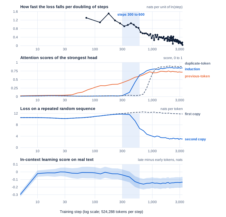
Across the 49 snapshots, the four measurements line up:
Swipe to pan the diagram, or tap it to zoom.
All four changes Olsson et al. use to define the phase change fall inside the same 300 steps, 157 to 315 million tokens.
The heads
Until step 300, no head scores above 0.03 on the induction test. At step 400 the best scores 0.13, at 500 0.42, at 600 0.63, and at 1,000 0.81. The three strongest are heads 8.9, 8.10 and 8.11. In grouped-query attention, every three query heads share one key-value head, and these three are exactly one group: they read the same keys and values and differ only in their queries. A fourth, 7.2, reaches 0.40 by the end.
The previous-token heads come first and grow slowly. The best one below layer 8 scores 0.11 at step 50, 0.36 at step 200, 0.41 (head 4.0) at step 300 and 0.57 at step 500, and by the end the strongest are 6.3 at 0.72 and 7.9 at 0.59. That’s the order Part 4’s circuit needs: an induction head can only match “the token whose previous token was A” after a previous-token head has written that information into the residual stream. The duplicate-token head comes last: no head scores above 0.04 at step 600, and then head 4.6 reaches 0.26 at step 800, 0.67 at step 1,000 and 0.87 at the end.
The behavior
On the repeated sequence, the loss on the second copy is 11.75 nats at step 300, as bad as the first copy, then 9.38 at step 500, 6.70 at step 600, 4.00 at step 1,000 and 2.96 at the end, while the first copy stays between 10.2 and 12.5 (95% confidence intervals within ±0.09). GPT-2 small’s second copy, in Part 4, cost 0.22: this model copies, but less sharply.
On real text, the in-context learning score is Olsson et al.’s, “the loss of the 500th token in the context minus the average loss of the 50th token in the context,” where negative means later tokens are easier. A single token’s loss is noisy (over 1,000 documents the 95% confidence interval is ±0.25 nats), so the numbers here use Part 4’s smoothed version: mean loss over tokens 491 to 510 minus tokens 41 to 60. Apart from a brief -0.30 at step 5 that this part didn’t trace, it sits near zero until step 300, where it reads -0.04 (±0.07), then -0.16 at step 700 and -0.14 (±0.07) at the end. Measured on the same documents, the change from step 300 to step 700 is -0.12 (±0.04), and the change from step 700 to the end is +0.03 (±0.03): it appears inside the band and then holds, as Olsson et al. found.
The amount is small. Olsson et al.’s models had “roughly 0.4 nats” after the phase change, and GPT-2 small’s smoothed gap in Part 4 was 0.64. Different text and tokenizers make these hard to compare, but this model gets less from its context.
The bump
Olsson et al. describe a small “bump” in the loss: “a period of visibly steeper improvement than the parts of the curve before and after.” Part 7’s loss curve looked smooth. The top panel above plots how fast the validation loss falls per unit of the logarithm of the step, which would decline steadily on a smooth power law. It falls to 0.91 between steps 300 and 350, rises back to 1.05 between 400 and 450, and then falls again. The 25-step average of the training loss, on different text, agrees: 0.88 over steps 300 to 400, then 1.02 over steps 400 to 500. That bump, about a tenth of a nat per unit of log step, is too small to see in the loss itself. An earlier rise, from 1.09 around step 120 to 1.51 around step 175, lines up with the end of warm-up at step 150; the later one comes during a smooth cosine decay, with nothing in the schedule to explain it.
Did the new heads cause it?
The scores above are correlations. To test cause, mean ablation replaces a head’s output with its average over held-out text, as in Part 4, so the head contributes its typical value but nothing about the current input. Each row ablates the three heads with the highest induction scores at that snapshot, ranked on a separate set of 100 sequences, and compares with 10 random sets of three heads drawn from outside the top 12. The in-context learning (ICL) columns use 500 held-out documents.
| Step | Top three heads | Second-copy loss: intact, top 3 ablated | ICL score, intact | Change from ablating the top 3 (95% CI) | Change from 3 random heads, median |
|---|---|---|---|---|---|
| 300 | 8.10, 8.8, 8.9 (scores ≤ 0.03) | 11.75, 11.86 | -0.045 | +0.008 (±0.006) | +0.001 |
| 400 | 8.10, 8.9, 8.11 | 11.61, 11.97 | -0.070 | +0.032 (±0.013) | +0.001 |
| 500 | 8.10, 8.9, 8.11 | 9.38, 12.03 | -0.155 | +0.108 (±0.025) | +0.001 |
| 600 | 8.10, 8.9, 8.11 | 6.70, 11.82 | -0.165 | +0.133 (±0.030) | +0.001 |
| 1,000 | 8.9, 8.10, 8.11 | 4.00, 11.20 | -0.161 | +0.137 (±0.032) | +0.000 |
| 3,360 | 8.9, 8.10, 7.2 | 2.96, 9.57 | -0.166 | +0.091 (±0.021) | +0.001 |
From step 500 on, three heads carry the copying: without them the second copy costs as much as the first. On real text, ablating them at steps 600 to 1,000 erases 75% to 85% of the in-context learning score, against almost nothing for random heads; at step 500, 70%. At step 3,360 the ranking puts 7.2 ahead of 8.11; ablating the top five, which include both, raises the ICL score by 0.153 (±0.036), about 92% of it, and the loss over all tokens by 0.18 nats, against 0.03 for the median random five.
The model has few backups: ablating its single best induction head at the end raises the second-copy loss from 2.96 to 5.20, where GPT-2 small’s best head, in Part 4, moved it from 0.22 to 0.27.

The stages overlap: previous-token heads were already growing while the bigram fit was still improving.
Step 4: smaller models, and Pythia
Does the timing follow the data, in tokens, or the training, in steps? Olsson et al. put their window at “roughly 2.5 to 5 billion tokens,” and Tigges et al. (2024) found that in Pythia models from 70 million to 2.8 billion parameters, “most models’ induction heads emerge soon after they have seen 2 × 10⁹ tokens.” This model formed them after 0.2 to 0.3 billion.
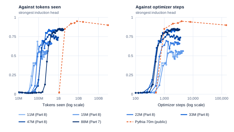
From Scratch Part 8’s size sweep can separate the two, because its models used different batch sizes: 65,536 tokens per step for the two smallest, 131,072 for 22M and 262,144 for 33M and 47M, each run with its own learning rate and a warm-up of 4.5% of its steps. Each saved 20 or 21 snapshots, one every 5% of the run. Pythia-70m adds a public model with 2,097,152 tokens per step; seven of its checkpoints were measured with Part 4’s code (TransformerLens 3.9.0, FP32, weight processing on, 200 repeated sequences from Part 4’s Pythia token set; 1.69 GB downloaded, Apache-2.0).
Swipe to pan the diagram, or tap it to zoom.
Plotted against tokens, the jumps spread over a factor of about 40. Plotted against steps, they bunch together.
| Model | Parameters | Tokens per step | Last snapshot with best head below 0.15 | First snapshot at or above 0.35 | Best induction head at the end | Second-copy loss at the end |
|---|---|---|---|---|---|---|
| From Scratch 11M | 10.9M | 65,536 | step 501 (33M tokens) | step 835 (55M) | 4.1: 0.52 | 6.24 |
| From Scratch 15M | 14.7M | 65,536 | step 675 (44M) | step 900 (59M) | 5.1: 0.56 | 5.48 |
| From Scratch 22M | 22.0M | 131,072 | step 504 (66M) | step 672 (88M) | 5.1: 0.66 | 3.10 |
| From Scratch 33M | 32.9M | 262,144 | step 252 (66M) | step 504 (132M) | 6.2: 0.83 | 2.83 |
| From Scratch 47M | 47.2M | 262,144 | step 360 (94M) | step 540 (142M) | 7.8: 0.74 | 3.04 |
| From Scratch 88M | 88.1M | 524,288 | step 400 (210M) | step 500 (262M) | 8.9: 0.84 | 2.96 |
| Pythia-70m | 70M | 2,097,152 | step 512 (1.07B) | step 1,000 (2.10B) | 3.6: 0.90 | 4.31 |
Each From Scratch second-copy loss has a 95% confidence interval within ±0.14 nats (200 sequences). Every model’s best head crossed from below 0.15 to above 0.35 somewhere between step 252 and step 1,000; in tokens, somewhere between 33 million and 2.1 billion. Part 8’s two equal-compute runs agree: the 22M model trained on a schedule less than half as long (1,507 steps, warm-up 68) crossed between steps 525 and 675, almost exactly where the full-length 22M run did, and the 11M model trained on a schedule nearly twice as long crossed between steps 606 and 909. In every From Scratch model, the best induction head sits in the last or second-to-last layer.
Smaller models end with weaker heads and copy worse. A head can also fade after it forms: in the 11M model trained nearly twice as long, the best score peaked at 0.45 around step 2,100 and ended at 0.28, with the second-copy loss back up to 8.05, while its in-context learning score on real text held at -0.19. Tigges et al. saw something similar in Pythia’s successor heads: “the behavior of these heads eventually decreases, while task performance does not.”
That doesn’t make steps what matters in general. The runs share one recipe (AdamW, a short warm-up, a cosine decay) with different learning rates, and Pythia formed its heads during its 1,430-step warm-up while the From Scratch runs had finished theirs within 68 to 273 steps. Olsson et al.’s small models used about a million tokens per step, so their 1 to 3 billion tokens was also roughly 1,000 to 3,000 steps. For these nine runs, the number of updates predicted formation far better than the amount of text.
Step 5: a feature over training
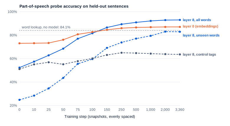
A representation is the other kind of structure: when does a property become readable from the model’s vectors? Part 3 trained part-of-speech probes, linear classifiers that read a word’s tag from one layer’s residual stream vector, on GPT-2 small. The same probes ran here on 12 snapshots, with Part 3’s data: Universal Dependencies English EWT v2.18 (CC BY-SA 4.0), 4,000 training sentences (64,014 words) and all 2,077 test sentences (24,386 words), 17 tags, each word read at its last token. Layer l is the residual stream entering block l; layer 10 is the last block’s output. Part 3’s control task gives every word type a random fixed tag, so the probe can only score by memorizing words.
Swipe to pan the diagram, or tap it to zoom.
Most of the readability arrives in the first 150 steps, before the induction heads.
| Step | Layer 0 (embeddings) | Layer 8 | Layer 8, words not seen in probe training | Layer 8, control tags |
|---|---|---|---|---|
| 0 | 73.1% | 52.3% | 24.8% | 51.1% |
| 50 | 76.1% | 68.5% | 43.5% | 55.1% |
| 150 | 84.6% | 86.5% | 69.2% | 63.1% |
| 500 | 86.6% | 90.9% | 77.1% | 64.7% |
| 3,360 | 87.1% | 93.0% | 82.9% | 63.6% |
Every accuracy has a 95% confidence interval within ±0.8 points (bootstrap over test sentences). The untrained model already scores 73% at layer 0, which is not knowledge: random embeddings give every word its own random vector, and a linear probe can memorize the tag of each word it has seen. Its control accuracy, 73.7%, says the same, and so does its 36% on unseen words. Training then makes the tags readable in a way memorization can’t explain: on unseen words, layer 8 goes from 25% to 69% by step 150 and 83% at the end.
The final model is close to GPT-2 small, which Part 3 measured at 94.4% at its layer 8 and 86.6% on unseen words, and above the 84.1% a word lookup scores without any model. The gap between layer 8 and the embeddings, the part that needs context, grows from 1.9 points at step 150 to 5.9 at the end. A probe measures what is readable; whether the model uses it would take an intervention.
In the real world
- Olsson et al. tracked 34 Transformers and found that in-context learning “develops abruptly in a narrow window early in training (roughly 2.5 to 5 billion tokens),” going from “less than 0.15 nats” to “roughly 0.4 nats,” and that one-layer models, which can’t compose two heads, never form induction heads. Their small models saw about 10 billion tokens in 10,000 steps, warmed up over the first 1.5 billion, and showed the phase change “at approximately 1-3 billion tokens.” Published results, not reproduced here.
- Hoogland et al. (2024) split the training of a two-layer attention-only model with about 3 million parameters into stages: it “first learns to predict using bigram statistics,” then “common n-grams,” then forms previous-token heads and then induction heads, the order measured above. Its bigram fit came within “only 0.3 nats” of the bigram entropy; this model’s came within 1.16, with a 32,768-token vocabulary and different data.
- Tigges et al. tracked circuits across 300 billion tokens of Pythia training and found that task abilities and the heads behind them “emerge consistently at similar token counts across scale”; every Pythia size uses the same 2-million-token step, so tokens and steps move together there.
- Chen et al. (2024) found the same kind of abrupt change in BERT-style masked language models: attention heads that track syntax form in “a brief window in pretraining,” together with “a steep drop in loss,” and suppressing them during training showed they were needed for the grammar that came later.
- Singh et al. (2024) clamped activations during training on synthetic data and identified “three underlying subcircuits that interact to drive IH formation, yielding the phase change”: one reason the jump is sudden is that the circuit pays off only once all its parts exist.
- Pythia published 154 checkpoints per model, log-spaced early, which is what makes comparisons like Step 4 possible without retraining anything.
Common misconceptions
- “Abilities grow as smoothly as the loss curve.” Induction heads went from a score of 0.03 to 0.63 in 300 steps, and in-context learning appeared with them. The loss curve shows only a small bump, invisible without plotting its slope.
- “The phase change happens at a fixed number of tokens.” In nine runs it happened between optimizer steps 250 and 1,000, while the tokens read by then ranged from 33 million to 2.1 billion. Token counts work as a rule of thumb only when the batch size is held fixed, as in Pythia.
- “What a model learns early, it keeps.” It is closest to the unigram model at step 50 and to the bigram model at step 150, then moves away from both: by the end its KL divergence from the unigram model is 4.98 nats, worse than the untrained model’s 2.95.
- “A probe on an untrained model reads nothing.” It read part of speech at 73% from random embeddings, by memorizing words. The control task and the unseen-word accuracy are what separate that from structure training built.
- “Induction heads are a GPT-2 quirk.” They formed in every From Scratch run and in Pythia-70m, with different sizes, batch sizes and learning rates, and in the 88M model three heads carry 75% to 85% of its in-context learning score once they form.
Key takeaways
- Saved weights turn interpretability into a time-lapse: the same measurements on 49 snapshots show what forms and when.
- The model fits word frequencies first, closest at step 50, then word pairs, closest at step 150, and then leaves both behind as it starts using longer context.
- Induction heads form abruptly between steps 300 and 600, after the previous-token heads they depend on and before a duplicate-token head. Copying loss drops from 11.8 to 6.7 nats, in-context learning appears, and the loss curve bends with a small bump.
- Ablation confirms the link: three heads that share one key-value group carry 75% to 85% of the in-context learning score between steps 600 and 1,000, and random heads carry almost none.
- Across eight From Scratch runs and Pythia-70m, induction heads appeared between optimizer steps 250 and 1,000, even though the tokens read by then differed by a factor of about 40.
What’s next
This part watched a model build its machinery. Part 11 asks what interpretability can do for safety: probes that try to catch deception and sycophancy, diffing a base model against its chat version to see what fine-tuning changed, and what auditors have found when they looked inside real models.
Further reading
- In-context Learning and Induction Heads (Olsson et al., 2022): the phase change, the in-context learning score and the loss bump; also on arXiv.
- Neural Networks Learn Statistics of Increasing Complexity (Belrose et al., 2024): the distributional simplicity bias, with n-gram tests on Pythia checkpoints.
- Loss Landscape Degeneracy and Stagewise Development in Transformers (Hoogland et al., 2024): bigram, n-gram, previous-token and induction stages in a small attention-only model.
- LLM Circuit Analyses Are Consistent Across Training and Scale (Tigges et al., 2024): when induction, name-mover and other heads emerge across Pythia sizes.
- What needs to go right for an induction head? (Singh et al., 2024): the subcircuits behind induction-head formation, found by clamping activations during training.
- Sudden Drops in the Loss: Syntax Acquisition, Phase Transitions, and Simplicity Bias in MLMs (Chen et al., 2024): an abrupt syntax-attention transition in BERT and what it enables.
- Pythia: A Suite for Analyzing Large Language Models Across Training and Scaling (Biderman et al., 2023): the public checkpoints used for the comparison in Step 4.
- A Mathematical Framework for Transformer Circuits (Elhage et al., 2021): why an induction head needs a previous-token head in an earlier layer.