
Inside the Model: Interpretability · Part 5 of 12
Activation Patching and Causal Tracing, Measured in GPT-2
Swap one activation between two prompts to find where GPT-2 tracks names and recalls facts, and measure how corruption and metric choices change the answer.
On this page
TL;DR
Activation patching runs a model on two prompts that differ in one detail, copies one internal activation from one run into the other, and measures how much of the answer follows the copy. That shows where the difference between the prompts is carried, layer by layer and head by head. This part uses it to recover most of the indirect-object circuit in GPT-2 small from 500 generated prompts, then runs causal tracing, the version that noises a subject’s embeddings, on Part 1’s landmark facts in GPT-2 small and Qwen2.5-0.5B. It also measures three choices that change the answer: Gaussian noise or a real replacement token, probability or logit difference, and whether the layer where a fact shows up in a trace is the best layer to edit it.
Why it matters
GPT-2 small reads “When Mary and John went to the store, John gave a drink to” and prefers ” Mary” over ” John” by 3.36 logits. Change the second “John” to “Mary” and it prefers ” John” by 2.48. Now take that second prompt and paste in one vector from the first run: the 768 numbers of the residual stream at the second name, entering block 0. The preference for ” Mary” comes back completely.
Paste the same position’s vector entering block 9 instead, and almost nothing comes back: 9% of the gap. Paste the last token’s vector entering block 9, and 97% comes back. Somewhere in blocks 8 and 9, the information that decides the answer moved from the second name to the end of the sentence, and the swap proves the model depends on it, which an attention pattern or a probe can’t.
That’s activation patching. Part 1 found that removing GPT-2’s first MLP costs more than any other layer on 168 landmark facts, and warned that a removal can’t say whether a layer stores a fact or just keeps the model working. Patching can tell, because it swaps in a real alternative instead of a blank.
The intuition
Picture two identical radios on a workbench, one tuned to news and one to music. You want to know which wire carries “which station”. So you unplug one wire in the music radio and plug in the matching wire from the news radio. If the music radio starts playing news, that wire carries the station. If nothing changes, it doesn’t, or not on its own.
Activation patching does the same with two prompts that differ in one detail. Because the prompts agree on everything else, any change in the answer has to come from that detail.
The analogy breaks in two places. A radio wire carries one signal, while one activation vector carries many pieces of information at once, and the swap moves all of them. And radio parts don’t react: in a model, every layer after the patch recomputes from the patched value, so later parts can undo the swap or amplify it.
Step 1: clean, corrupted, patched
Every patching experiment has three runs: a clean prompt that gets the behavior right, a corrupted prompt that changes one detail so the answer changes, and a patched run, one of the two with a single activation copied in from the other.

The direction matters, as Heimersheim and Nanda (2024) stress. Denoising runs the corrupted prompt and pastes in clean activations, so it finds activations sufficient to restore the behavior. Noising runs the clean prompt and pastes in corrupted activations, so it finds activations necessary for it. If two parts must both be clean (an AND), denoising either one alone does nothing while noising either one breaks the output; if either part is enough (an OR, such as a backup head), it’s the other way round.
The metric: logit difference
The score is the logit difference, the logit (the raw score before softmax, from Fundamentals Part 4) of the right name minus the logit of the wrong one. Each run’s value is turned into a share of the gap:
share restored = (LD_patched - LD_corrupted) / (LD_clean - LD_corrupted)With the numbers above, a patch that brings the logit difference to +1.0 restores (1.0 - (-2.48)) / (3.36 - (-2.48)) = 0.60 of the gap. Heimersheim and Nanda give the reason to prefer this metric: the residual stream is a sum of component outputs, and the logit difference is, up to the final layer norm, a linear function of that sum, so each component can shift it by a fixed amount. It also cancels anything that boosts both names equally, such as a “a name comes next” signal. Probability is exponential in the logits, so the same push of +2 logits can move it by 1 or 40 percentage points depending on where it started.
Here is the whole experiment for one prompt, using TransformerLens 3.9.0 on GPT-2 small (124 million parameters, MIT license, openai-community/gpt2) in fp32 on an NVIDIA GeForce RTX 4060 Laptop GPU (8 GB):
from functools import partial
import torch
from transformer_lens import HookedTransformer

torch.set_grad_enabled(False)
model = HookedTransformer.from_pretrained("gpt2", device="cuda")   # fp32, LayerNorm folded
clean = "When Mary and John went to the store, John gave a drink to"
corrupt = "When Mary and John went to the store, Mary gave a drink to"
mary, john = model.to_single_token(" Mary"), model.to_single_token(" John")

def logit_diff(logits):                     # Mary minus John, at the last position
    return (logits[0, -1, mary] - logits[0, -1, john]).item()

clean_logits, cache = model.run_with_cache(clean)
ld_clean, ld_corrupt = logit_diff(clean_logits), logit_diff(model(corrupt))
s2 = [i for i, t in enumerate(model.to_str_tokens(clean)) if t == " John"][1]
print(f"clean {ld_clean:+.2f}, corrupted {ld_corrupt:+.2f}, S2 at position {s2}")

def patch(act, hook, pos):                  # paste the clean activation at one position
    act[:, pos] = cache[hook.name][:, pos]
    return act

for layer in (0, 6, 8, 9, 10):
    row = []
    for name, pos in (("S2", s2), ("END", -1)):
        hook = (f"blocks.{layer}.hook_resid_pre", partial(patch, pos=pos))
        ld = logit_diff(model.run_with_hooks(corrupt, fwd_hooks=[hook]))
        row.append(f"{name} {(ld - ld_corrupt) / (ld_clean - ld_corrupt):.2f}")
    print(f"block {layer:2d}:", *row)
clean +3.36, corrupted -2.48, S2 at position 10
block 0: S2 1.00 END 0.00
block 6: S2 0.93 END -0.00
block 8: S2 0.63 END 0.33
block 9: S2 0.09 END 0.97
block 10: S2 0.03 END 1.02hook_resid_pre of block l is the residual stream entering that block. from_pretrained applies TransformerLens’s weight processing (LayerNorm folded into the next weights, weights that write to the stream centered), which leaves outputs unchanged; every GPT-2 number here uses it.
Step 2: finding the IOI circuit by patching
The task is indirect object identification (IOI) from Wang et al. (2022): in “When Mary and John went to the store, John gave a drink to”, the indirect object (IO) is Mary, the subject (S) is John, and S1 and S2 are the subject’s first and second mentions. Wang et al. found 26 attention heads in 7 classes that do it.
The prompt set is generated from Wang et al.’s 15 templates (Appendix E), each in its BABA order and the ABBA variant with the first two names swapped: 500 prompts, from 110 single-token first names, 20 places and 20 objects (seed 0). GPT-2 small prefers IO over S on 98.8% of them, with a mean logit difference of 3.87 (95% bootstrap confidence interval 3.72 to 4.03) and P(IO) of 51%. Wang et al. report 3.56, 99.3% and 49% over 100,000 prompts. The main corruption is symmetric token replacement (STR) on S2: the second mention becomes the IO name, as in the listing, which flips the mean logit difference to -3.83. Intervals below are 95% bootstrap intervals over prompts; every one quoted for a head is within ±0.04.
Layer by position
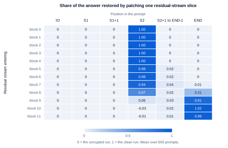
Swipe to pan the diagram, or tap it to zoom.
Over 500 prompts, at block 8 the stream at S2 restores 0.67 (0.65 to 0.68) and at END 0.31; by block 9 END restores 0.91. Positions before S2 restore exactly 0, because GPT-2 reads left to right and those tokens are identical in the two prompts. Patching only finds what the two prompts make different.
Splitting blocks into attention and MLP outputs shows what moves it. Patching attention layer 8’s output restores 0.55 (0.53 to 0.56) of the gap, 0.53 from the END position alone; layer 7 restores 0.32 and layer 9 0.25. MLP 0 restores 0.87 when patched at all positions and 0 at END only, because it acts on S2’s token itself, as part of the embedding. No other MLP passes 0.10, so the heads do the moving.
Head by head
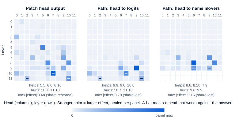
Patching each of the 144 heads’ outputs at every position gives the left panel below; the other two panels use path patching.
Swipe to pan the diagram, or tap it to zoom.
Ordinary patching finds the right heads but mixes their roles: induction head 5.5 (0.33 of the gap), S-inhibition heads 8.6 (0.29), 8.10 (0.27) and 7.9 (0.21), name mover 9.9 (0.18), and two heads that push the wrong way, 10.7 (-0.48) and 11.10 (-0.26). Name movers 9.6 and 10.0 barely register. This sweep can’t say which heads write the answer and which steer the writers.
Path patching, introduced by Wang et al., tests one connection at a time. It runs the clean prompt, swaps one sender head’s output for its value on a prompt with three unrelated names (Wang et al.’s ABC prompts), freezes every other head at its clean value, and lets the change reach only chosen receivers. The table gives the change in logit difference as a share of the clean value; negative means the path carries the answer.
| Path patched (sender → receiver) | Heads that matter most | Change in logit difference |
|---|---|---|
| head → logits, at END | 9.9, 9.6, 10.0 | -79%, -32%, -22% |
| same | 10.7, 11.10 | +51%, +26% |
| head → queries of 9.9, 9.6 and 10.0, at END | 8.6, 8.10, 7.9, 7.3 | -16%, -11%, -9%, -5% |
| head → values of 7.3, 7.9, 8.6 and 8.10, at S2 | 5.5, 6.9, 3.0, 0.1 | -38%, -14%, -13%, -5% |
Each row recovers Wang et al.’s classes in their order of discovery: the three name movers that write the name into the logits, the two negative name movers that write against it, exactly the four S-inhibition heads that steer the name movers’ queries, and the induction heads 5.5 and 6.9 and duplicate-token heads 3.0 and 0.1 that feed the S-inhibition heads at S2, heads Part 4 found by attention scores.
The name movers put 0.63 of their attention from END on IO in the clean prompts (Wang et al.: 0.59) and 0.63 on S1 in the STR prompts, so the corruption swaps which name they read without breaking them. Denoising and noising gave nearly the same head list (5.5 at 0.33 restored, 0.34 destroyed), so this task’s main heads act in series, not as backups.
Step 3: causal tracing for factual recall
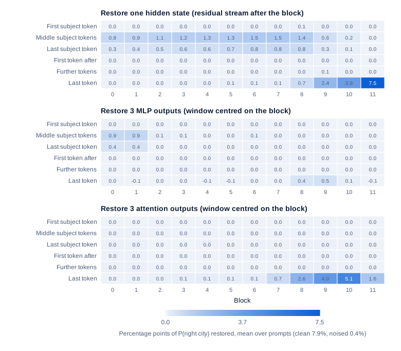
Causal tracing is the patching variant Meng et al. (2022) used to find where GPT-2 XL recalls facts, the basis of ROME (Rank-One Model Editing). There is no second prompt: the corrupted run adds Gaussian noise to the subject’s token embeddings (three times their standard deviation), and the patched run restores one hidden state, the residual stream after one block at one position, from the clean run. The score, the average indirect effect, is the probability of the right answer brought back, averaged over prompts and noise draws. MLP and attention outputs were restored in windows of 10 adjacent layers, because single layers did little.
On 1,000 facts GPT-2 XL knew, the noise cut the answer’s probability from 27.0% to 8.47%. One hidden state at the subject’s last token at layer 15 brought back 8.7 points, and MLP windows there 6.6 points against 1.6 for attention: the “early site”. The “late site” is at the last token, carried by attention.
Our run uses the 67 of Part 1’s 168 landmark prompts (“The Eiffel Tower is located in the city of”) where GPT-2 small ranks the right city first among 54, with 10 noise draws each and 3-layer windows, about the same fifth of the depth as Meng et al.’s 10 of 48. The noise cuts P(right city) from 7.9% (5.7 to 10.3%) to 0.4%.
Swipe to pan the diagram, or tap it to zoom.
GPT-2 small shows both sites. The subject’s tokens carry the answer through block 8: restoring the last subject token’s hidden state after block 7 recovers 11% (7 to 17%) of the lost probability, and the middle subject tokens, such as “iff” in “The Eiffel Tower”, recover 20%. After block 8 that drops to 3%, while the last token climbs from 10% to 50% between blocks 8 and 10. Attention at the last token carries this late site: the window centred on block 10 restores 69%.
The early site differs from GPT-2 XL’s. The MLP windows at the subject’s last token restore 5.5% around blocks 0 and 1 and nothing after; a single MLP, MLP 0, restores 3.8%, and no other single MLP restores more than 0.2%. Meng et al.’s severed test points the same way: restoring the last subject token’s hidden state after blocks 0 to 2 while freezing every later MLP at that token at its noised value drops the effect from 4.4 to 6.4% to between 0.6 and 1.7%, while freezing the attention outputs instead leaves 2.9 to 6.0%. The subject’s representation depends on MLPs, but in GPT-2 small on the first two or three.
Part 1’s question: storage or support?
Part 1 mean-ablated MLP 0 at every position after the start token and lost 1.17 logits of the right city’s lead over the other 53, and warned that MLP 0 might only be keeping every token’s representation working. Splitting the same ablation by position settles it. Mean-ablating MLP 0 only at the template’s tokens (” is located in the city of”) costs 0.002 logits (-0.006 to 0.010); only at the landmark’s tokens, 1.16 (0.91 to 1.38). Patching agrees: swapping in MLP 0’s output from a different landmark’s prompt costs -0.005 logits at the template’s positions and 1.86 (1.46 to 2.29) at the subject’s.
The cost is specific to the landmark’s tokens. With symmetric replacement (each prompt paired with another known landmark of the same token length from a different city, 67 pairs), patching MLP 0’s output at the last subject token alone restores 16% (11 to 21%) of the gap between the two cities. That fits MLP 0 building the landmark’s identity from its tokens, part of what Geva et al. (2023) call subject enrichment. It doesn’t show MLP 0 stores “Paris”: in these pairs the landmark and the city change together, so patching can’t separate them.
Other models
The same run on Qwen2.5-0.5B (494 million parameters, Apache-2.0, Qwen/Qwen2.5-0.5B) used from_pretrained_no_processing in fp32, 5 noise draws per prompt and 5-layer windows for its 24 blocks. Qwen has no start token, so its <|endoftext|> is prepended to keep position 0 out of the noised subject.
| Causal tracing on the landmark facts | GPT-2 small (12 blocks) | Qwen2.5-0.5B (24 blocks) |
|---|---|---|
| Facts known (of 168) | 67 | 135 |
| P(right city): clean, then noised | 7.9%, then 0.4% | 43.2%, then 0.2% |
| Best hidden state at the last subject token | 11% (7 to 17%), after block 7 | 40% (32 to 48%), after block 5 |
| Best MLP window at the last subject token | 6% (3 to 10%), blocks 0 to 2 | 21% (15 to 27%), blocks 2 to 6 |
| Best attention window at the last token | 69% (62 to 76%), blocks 9 to 11 | 32% (28 to 35%), blocks 17 to 21 |
| MLP 0 mean-ablated: logits lost at subject tokens | 1.16 (0.91 to 1.38) | 8.71 (8.11 to 9.28) |
| Same, at template tokens | 0.002 | -0.009 |
Percentages are shares of the lost probability restored. Qwen, which knows the facts far better, shows Meng et al.’s early site clearly: an MLP band in its first quarter at the subject’s last token, then a hand-off to the last token through attention in blocks 17 to 21. Its large MLP 0 cost, 8.73 logits in Part 1, again comes entirely from the landmark’s tokens.
Step 4: the choices that change the answer
Zhang and Nanda (2023) varied the corruption and the metric on these tasks and found the conclusions moved. We measured both, plus one claim from editing.
Gaussian noise versus a real alternative
Gaussian noise (GN) builds an input no model has seen, while STR builds one it could meet in training. On IOI, noising S2’s embedding (three times the name embeddings’ spread) leaves GPT-2 at 9% for each name and changes how the circuit runs: the name movers’ attention from END, 0.63 on IO in the clean run, becomes 0.25 on IO and 0.21 on S1. Zhang and Nanda measured 0.58, then 0.26 and 0.21 with GN. Under GN, induction head 5.5’s patching effect falls from 0.33 to 0.12, and duplicate-token head 0.10, which helps on clean prompts, shows up as harmful (-0.06 in probability), the same anomaly Zhang and Nanda report for 0.10.
On the landmark facts, the two corruptions agree more than Zhang and Nanda’s GPT-2 XL runs did, where GN’s MLP peak was 2 to 5 times STR’s. Measured on the same metric (the right city’s lead over the other 53, as a share of the gap), the best MLP window at the last subject token restores 16% under GN and 15% under STR in GPT-2 small. In Qwen it restores 34% under GN and 23% under STR, and 21% against 14% in probability: GN’s peak is 1.5 times STR’s, the same direction as Zhang and Nanda’s finding but smaller. The noise cut P(right city) to 0.2 to 0.4%, so in both models every restoration starts from the floor.
Probability versus logit difference
Probability can’t go below zero, so once the corrupted run has driven the right answer close to zero it can’t register a head that pushes the wrong way. STR leaves P(IO) at 2.6%. Under the detection rule of Zhang and Nanda (an effect more than 2 standard deviations from the mean over heads), logit difference flags both negative name movers, 10.7 at -0.48 and 11.10 at -0.26; probability flags neither, scoring them -0.05 and -0.03. Zhang and Nanda found probability missed 11.10 under the same corruption. With the ABC corruption, which drives P(IO) to 0.07%, probability finds only 9.9 of all the heads, while logit difference finds all three name movers and both negative ones.
The two metrics also disagree on size. Restored after block 7, GPT-2’s middle subject tokens recover 41% of the lost probability but 30% of the logit-difference gap under STR, so which positions look important depends on the metric, as Zhang and Nanda found for GPT-2 XL.
Does localization tell you where to edit?
ROME used causal tracing to choose which MLP to edit. Hase et al. (2023) tested whether the trace predicts where edits succeed, on 652 facts in GPT-J (6 billion parameters). It doesn’t: the edited layer explains 94.7% of the variance in ROME’s edit success, and adding each fact’s tracing effect raises that to 94.8%. At ROME’s default layer the correlation was -0.13.
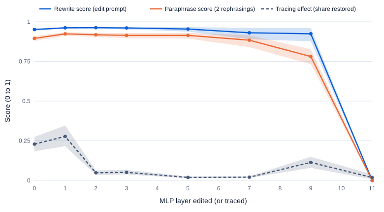
We ran a small version on GPT-2 small: for each of the 67 known facts, a ROME-style rank-one edit of MLP W_out at one of 8 layers sends the landmark to a random other city, 536 edits in all. (The target vector comes from 20 Adam steps without ROME’s KL term; the key covariance from 100,000 FineWeb-Edu tokens, ODC-By 1.0, plus a small ridge.) Each edit gets Hase et al.’s rewrite score, how far the new city’s probability moved toward 1 on the edited prompt, and paraphrase score, the same on two rephrasings.
Swipe to pan the diagram, or tap it to zoom.
The trace peaks at MLP layer 1 for 35 of the 67 facts, yet edits at layers 3 and 5, where it is near 0.05 and 0.02, generalize to the rephrasings as well (0.91, against 0.92 at layer 1). The layer explains 92.6% of the variance in rewrite score, and adding the tracing effect adds 0.02 percentage points; within each layer, the correlation between the two lies between -0.04 and 0.07. Only layer 11 fails, because an edit at the subject’s token after the last attention layer can’t reach the final position. This is a reimplementation on a small model, but the pattern matches Hase et al.’s.
In the real world
- Wang et al.’s IOI circuit is 26 heads in 7 classes; run alone, it achieves 87% of the full model’s logit difference. Its backup name movers take over when the main ones are knocked out, an OR that a single noising sweep undercounts.
- Meng et al. used causal tracing on GPT-2 XL to pick the layer ROME edits, and MEMIT scaled editing to thousands of facts at once in GPT-J and GPT-NeoX. Not reproduced here.
- Conmy et al. (2023) automated the patching loop as ACDC, which kept 68 of GPT-2 small’s 32,000 edges for its greater-than task, all of them found earlier by hand. Part 8 covers this.
- Todd et al. (2023) used the same analysis to find a few attention heads that carry a “function vector” for an in-context task. Not reproduced here.
Common misconceptions
- “Patching tells you where a fact is stored.” It tells you where the difference between two prompts is carried. Edits worked as well at layers where the trace was near zero as at its peak.
- “Denoising and noising are the same test run backwards.” Denoising finds what is sufficient, noising what is necessary. They agreed on IOI’s main heads, which act in series, and disagree for ANDs and backups.
- “Any corruption will do.” Gaussian noise moved GPT-2’s name movers’ attention from 0.63 on the right name to 0.25 and made a helpful head look harmful. Swapping in a real name kept the circuit’s behavior intact.
- “Probability is the natural metric.” Once the corrupted answer is near zero, probability can’t register a head that pushes against it: it missed both negative name movers that logit difference found.
- “Patching every head finds the circuit.” It found 5.5, 8.6 and 9.9 but hid name movers 9.6 and 10.0. Path patching separated the heads that write the answer from the heads that steer them.
Key takeaways
- Activation patching copies one activation between a clean and a corrupted run and measures the share of the answer that follows. It is causal evidence about the detail the two prompts differ in, and only that.
- On 500 IOI prompts, the deciding information sits at the second name until block 8 and at the last token from block 9; path patching then recovered five of Wang et al.’s seven head classes, each by the connection it uses.
- Causal tracing finds Meng et al.’s two sites, with GPT-2 small’s subject MLP effect in blocks 0 and 1, and Part 1’s MLP 0 cost comes entirely from the landmark’s own tokens.
- The choices change the answer: Gaussian noise disturbed the circuit it was measuring, and probability missed heads that logit difference found.
- Where a trace peaks is a poor guide to where an edit works, in Hase et al.’s GPT-J study and in our GPT-2 edits.
What’s next
Patching treats a layer or a head as the unit, but one activation vector holds far more features than it has dimensions. Part 6 reproduces Anthropic’s toy models of superposition on the laptop: how a network packs more features than neurons, when it does and when it drops them, and why that makes single neurons such a poor unit for explanations.
Further reading
- How to use and interpret activation patching (Heimersheim & Nanda, 2024): denoising versus noising, AND and OR circuits, and why to trust logit difference.
- Towards Best Practices of Activation Patching in Language Models: Metrics and Methods (Zhang & Nanda, 2023): Gaussian noise versus symmetric token replacement, probability versus logit difference, sliding windows.
- Interpretability in the Wild: a Circuit for Indirect Object Identification in GPT-2 small (Wang et al., 2022): the IOI task, its templates, path patching and the 26-head circuit.
- Locating and Editing Factual Associations in GPT (Meng et al., 2022): causal tracing, the early and late sites, and ROME.
- Does Localization Inform Editing? (Hase et al., 2023): tracing effects explain almost none of the variance in edit success.
- Mass-Editing Memory in a Transformer (Meng et al., 2022): MEMIT, thousands of edits at once.
- Dissecting Recall of Factual Associations in Auto-Regressive Language Models (Geva et al., 2023): subject enrichment and attribute extraction.
- Towards Automated Circuit Discovery for Mechanistic Interpretability (Conmy et al., 2023): ACDC, patching automated over a whole graph.
- Function Vectors in Large Language Models (Todd et al., 2023): causal mediation analysis on in-context learning.
- TransformerLens: the hooks used for every patch here.