
Inside the Model: Interpretability · Part 12 of 12
Limits and Open Problems in Interpretability
The series in review: every part's headline result, a robustness audit of three of them, the field's sharpest critiques, and the problems still open.
On this page
TL;DR
This finale asks which of the series’ results deserve trust. It collects every part’s headline measurement in one table, then reruns three of them with one condition changed: new sentences for Part 1’s landmark facts, new inputs for Part 4’s induction heads, new kinds of text for Part 7’s sparse autoencoder. Then it covers the field’s sharpest critiques and the open problems a 29-author survey lists. By the end you’ll know which kinds of interpretability claims hold up, which don’t yet, and what it would take to say we understand a model.
Why it matters
In April 2025, Anthropic’s chief executive Dario Amodei wrote that the company has “a goal of getting to ‘interpretability can reliably detect most model problems’ by 2027.” Eight months later, the interpretability team at Google DeepMind wrote that “grand goals like near-complete reverse-engineering still feel far out of reach”, and that it had pivoted “from ambitious reverse-engineering to a focus on pragmatic interpretability.”
Both groups run the same methods this series ran on GPT-2, Qwen and Gemma. So which is it: a field two years from a working safety tool, or one that has lowered its sights?
It depends on which result you pick, and whether it survives a change of conditions. This part rechecks three of the series’ own results. The mechanisms held: the same five attention heads in GPT-2 came out on top under four new kinds of input. The rankings between close competitors didn’t: Part 7’s sparse autoencoder, trained on a laptop, beat OpenAI’s on the text it was trained on and lost to it on three of four other kinds of text.
The intuition
Think of reverse-engineering a program you only have as a compiled binary. You can watch its registers while it runs (the logit lens, probes), patch bytes and see what breaks (ablation, patching), or run a decompiler that turns machine code into something like source code (sparse autoencoders, attribution graphs): readable, mostly right, with blocks it couldn’t translate.
Engineers who do this trust the traces and the patches, and treat decompiler output as a draft to check.
The analogy breaks here. A binary was compiled from real source code, so a perfect decompilation exists, even if you never see it. Nobody wrote a model’s source. There may be no list of “true features” for a sparse autoencoder to recover, and no ground truth to grade an explanation against, which is the root of several open problems below.
Step 1: the series in one table
Each part ran its own experiment on a laptop GPU and reported numbers with a spread. The table collects the headline from each. The evidence column uses Part 1’s distinction: correlational methods read what is there, causal methods change something and watch the output.
| Part | Question | Headline result (measured here) | Evidence |
|---|---|---|---|
| 1 | Where does GPT-2 get the city for a landmark? | Attribution credits late attention heads; mean-ablating MLP 0, which writes nothing toward the answer, costs the most, 1.17 logits. Attribution and ablation rank the 24 layers alike at 0.69 in GPT-2 small but 0.16 in Qwen2.5-0.5B | Both |
| 2 | Can you read a half-finished prediction? | After block 6 of 12, the logit lens matches GPT-2’s final top token on 15.0% of 155,040 positions; a tuned lens trained in 6 minutes matches 45.2% | Correlational |
| 3 | What can a linear classifier read from a layer? | Part of speech at 94.4% against an 84.1% word lookup; truth of city facts at 78.4% (GPT-2) and 94.7% (Qwen, layer 9), falling to 59.1% and 68.8% on a rephrased sentence | Correlational, plus one nudge |
| 4 | Which heads copy repeated text? | Mean-ablating 5 of GPT-2’s 144 heads raises the loss on a repeated random sequence from 0.22 to 5.48 nats (5 random heads: 0.25); the top 12 carry 18% to 27% of in-context learning on WikiText | Causal |
| 5 | Where is the difference between two prompts carried? | On 500 IOI prompts the deciding information moves from the second name to the last token between blocks 8 and 9; editing a fact works as well at layers the trace ignores | Causal |
| 6 | Can a model store more features than dimensions? | A 5-dimensional toy kept 14 of 20 sparse features where a linear one kept 5; 75% of GPT-2’s rarely firing neurons split their firings across unrelated kinds of text | Toy models, then correlational |
| 7 | Can an SAE pull out readable features? | A 24,576-latent TopK SAE on GPT-2’s layer 8 explains 84.9% of the variance and raises the loss by 0.114 nats; 66% of 50 random Gemma Scope latents read clearly; clamping one moved at most 4 of 20 completions | Both |
| 8 | Can a graph trace one prompt’s computation? | Editing six Texas and five California features turned Gemma’s ” Austin” (41%) into ” Sacramento” (27%), but the transcoders miss 42% of an average MLP’s variance and the graph ranked single-node effects at only 0.29 | Both |
| 9 | Can you steer a model by adding a direction? | Ablating one difference-of-means direction cut Qwen2.5-1.5B-Instruct’s refusals of 100 held-out harmful requests from 99% to 11% for 0.01 nats on web text; adding it made the model refuse 98% of harmless requests and halved its quiz accuracy. For Egypt in Gemma 2 2B, a mean difference steered about twice as well as an SAE latent | Causal |
| 10 | What does training build, and when? | In 49 snapshots of the From Scratch 88M model, the unigram fit peaked at step 50 and the bigram fit at 150; induction heads switched on between steps 300 and 600 (best score 0.03 to 0.63) with in-context learning and a small loss bump, and ablating three heads removed 75% to 85% of that in-context learning. Nine runs formed them between steps 250 and 1,000 while their token counts differed about 40-fold | Correlational and causal |
| 11 | Can interpretability catch unsafe behavior? | Gemma 2 2B IT matched users’ stated opinions on 94% of NLP-survey questions but dropped only 1.8% to 3.9% of known facts under pressure. A lie probe caught 100% of held-out instructed lies at a 1% false-alarm rate, even when told to hide, yet flagged 63% of honest mistakes: it learned “probably false”, not intent. A base-model SAE transferred to the chat model at no higher splice cost | Both |
Two patterns show. The cleanest results are the narrowest: one behavior, one model, a causal test with a control. Five heads in GPT-2 carry copying of random tokens; six features carry “Texas” on one prompt. The broad claims, about what a layer represents or what a feature means, come with the largest caveats: probes that fall 19 to 26 points when a sentence is rephrased, feature labels that still fit at ordinary strengths for only a quarter of sampled latents.
The second is the gap between reading and using. In Part 1, attribution and ablation disagree about which layer matters most. In Part 3, Qwen’s truth direction was readable from layer 8 on but moved the answer mainly at layers 13 and 14. In Part 5, edits worked at layers the trace said were empty. Every time a reading method and an intervention were compared, they diverged somewhere.
Step 2: a robustness audit
A result measured once, on one prompt set with one seed, can be a fact about the model or about the setup. So this part reran three headline measurements with one condition changed and everything else (models, code, metrics) kept the same.
All three ran on an NVIDIA GeForce RTX 4060 Laptop GPU (8 GB) with PyTorch 2.11, TransformerLens 3.9.0 and SAELens 6.54.12. GPT-2 small (openai-community/gpt2, MIT license) ran in fp32 with TransformerLens weight processing on, as in the original parts; Qwen2.5-0.5B (Qwen/Qwen2.5-0.5B, Apache-2.0) in fp32 without weight processing, as in Part 1. Each audit first reproduced its part’s original number from the same code before changing anything. The helpers live in a small shared module, lab/replicate.py. The whole audit took 17 minutes of GPU time.
Audit 1: Part 1’s landmark facts, with new sentences
Part 1 asked where GPT-2 small gets the city in “The Brandenburg Gate is located in the city of”, over 168 landmarks. Direct logit attribution (DLA), which splits the answer into what each layer wrote, credited late attention layers. Mean ablation, which replaces a layer’s output with its average and reruns, found that MLP 0, the first block’s two-layer network, cost the most: 1.17 logits of the right city’s lead over the 53 others, while writing 0.01 logits directly.
The audit changed the sentence to “[landmark] is a famous landmark in the city of” and “If you want to see [landmark], you have to travel to the city of”, with the averages recomputed per sentence position. Intervals are 95% bootstrap intervals over the 168 prompts.
| Model and sentence | Right city ranked first of 54 | Cost of removing MLP 0 (logits) | Rank correlation of the two methods, 24 or 48 layer outputs | Layers in both top-5 lists |
|---|---|---|---|---|
| GPT-2, “is located in the city of” (Part 1) | 39.9% | 1.17 (0.92 to 1.39) | 0.69 (0.54 to 0.81) | 4 |
| GPT-2, “is a famous landmark in” | 39.9% | 1.41 (1.12 to 1.68) | 0.64 (0.49 to 0.78) | 4 |
| GPT-2, “If you want to see …” | 39.3% | 0.78 (0.60 to 0.97) | 0.77 (0.59 to 0.82) | 4 |
| Qwen, “is located in the city of” (Part 1) | 82.7% | 8.73 (8.16 to 9.30) | 0.16 (0.03 to 0.26) | 0 |
| Qwen, “is a famous landmark in” | 80.4% | 9.48 (8.88 to 10.07) | 0.15 (0.01 to 0.26) | 0 |
| Qwen, “If you want to see …” | 81.5% | 8.87 (8.32 to 9.39) | 0.16 (0.06 to 0.27) | 0 |
The first rows reproduce Part 1. The qualitative findings hold under both new sentences: DLA gives MLP 0 about 0.01 logits while removing it costs a large share of the answer, and on Qwen the two methods share none of their top five layers.
One headline didn’t hold. Part 1 said MLP 0 was GPT-2’s single most costly layer. With the “travel” sentence its cost falls by 0.38 logits (0.20 to 0.56, paired over the same landmarks), from 33% of the logit difference to 24%, and attention layer 9, at 1.04, takes first place.
Audit 2: Part 4’s induction heads, with new inputs
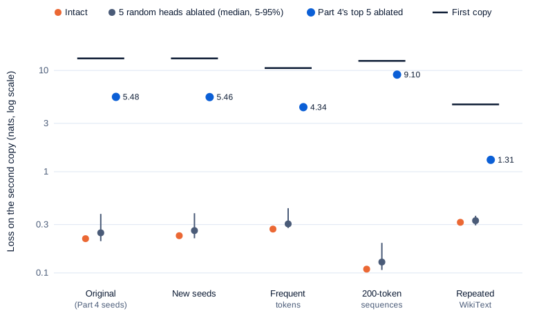
Part 4 found GPT-2 small’s five strongest induction heads, which find an earlier copy of the current token and predict what followed it, on 50 random tokens repeated twice. Mean-ablating them raised the loss on the second copy from 0.22 to 5.48 nats, against 0.25 for five random heads.
The audit changed the input four ways: new seeds; tokens drawn from WikiText-103’s 2,000 most frequent; 200-token sequences; and real 50-token WikiText-103 passages (CC BY-SA 4.0) shown twice. Each condition re-ranked all 144 heads on 200 sequences, then measured on 500 fresh ones (200 for the long ones), against 20 random sets of five heads from outside Part 4’s top 12. The new-seed check runs as shown:
import torch
from transformer_lens import HookedTransformer

torch.set_grad_enabled(False)
model = HookedTransformer.from_pretrained("gpt2", device="cuda")   # fp32, LayerNorm folded
top5 = [(5, 5), (6, 9), (7, 10), (5, 1), (7, 2)]                   # Part 4's induction heads

def repeated(seed, n=200, half=50):                                # [BOS] + r + r, as in Part 4
    g = torch.Generator().manual_seed(seed)
    r = torch.randint(1000, 49257, (n, half), generator=g)
    return torch.cat([torch.full((n, 1), 50256), r, r], 1).cuda()

ref, test = repeated(103), repeated(102)                           # new seeds; Part 4 used 3 and 2
_, cache = model.run_with_cache(ref, names_filter=lambda n: n.endswith("hook_z"))
mean_z = {l: cache[f"blocks.{l}.attn.hook_z"].mean((0, 1)) for l in range(12)}

def ablate(z, hook):                                               # replace each head's output by its mean
    for l, h in top5:
        if hook.layer() == l:
            z[:, :, h] = mean_z[l][h]
    return z

for name, hooks in [("intact", []), ("top-5 ablated", [(f"blocks.{l}.attn.hook_z", ablate) for l in (5, 6, 7)])]:
    logits = model.run_with_hooks(test, fwd_hooks=hooks)
    loss = -logits.log_softmax(-1)[:, :-1].gather(-1, test[:, 1:, None])[..., 0]
    print(f"{name}: first copy {loss[:, 1:50].mean():.2f}, second copy {loss[:, 51:].mean():.2f} nats")
intact: first copy 13.13, second copy 0.24 nats
top-5 ablated: first copy 12.97, second copy 5.40 natsThe listing uses 200 test sequences; the full audit used 500 per condition:
Swipe to pan the diagram, or tap it to zoom.
| Condition | Same 5 heads ranked top? | Second-copy loss, intact | Top 5 ablated (95% CI) | 5 random heads, median | Share of the repeat benefit removed |
|---|---|---|---|---|---|
| Original seeds (Part 4) | yes | 0.22 | 5.48 (5.43 to 5.54) | 0.25 | 41% |
| New seeds | yes | 0.23 | 5.46 (5.40 to 5.51) | 0.26 | 41% |
| Frequent tokens | yes | 0.27 | 4.34 (4.29 to 4.39) | 0.31 | 39% |
| 200-token sequences | yes | 0.11 | 9.10 (9.05 to 9.15) | 0.13 | 73% |
| Repeated WikiText | yes | 0.32 | 1.31 (1.29 to 1.34) | 0.33 | 23% |
The last column is the share of the drop from first-copy to second-copy loss that the ablation undoes. Every re-ranking picked exactly Part 4’s five heads, and no random set of five raised the loss above 0.51 nats, so the result held.
Its size depends on the input. On real text their induction scores fall from 0.83 to 0.93 down to 0.65 to 0.86, and ablating them undoes only 23% of the repeat’s benefit, since real text offers other cues. On long sequences it undoes 73%.
Audit 3: Part 7’s sparse autoencoder, on new kinds of text
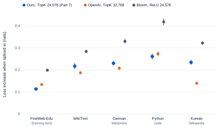
Part 7 trained a TopK sparse autoencoder (SAE) with 24,576 latents on GPT-2’s layer 8 using FineWeb-Edu. Splicing its reconstruction into the model raised the loss by 0.114 nats, slightly better than OpenAI’s public TopK SAE (0.134) and Joseph Bloom’s public ReLU SAE (0.199), with a warning about home advantage.
The audit ran the same three SAEs on four other kinds of text: 1,200 windows of WikiText-103 from 119 articles, and Part 6’s 400-window samples of German Wikipedia, Korean Wikipedia (both CC BY-SA 4.0) and CPython standard-library code (PSF License), each window 127 tokens after the start token. Intervals resample articles for WikiText and windows for the others, which makes those slightly narrow.
Swipe to pan the diagram, or tap it to zoom.
| Text | Ours minus OpenAI, loss increase (paired, nats) | Ours minus Bloom | Variance explained: ours / OpenAI |
|---|---|---|---|
| FineWeb-Edu (537,337 tokens) | -0.020 (-0.024 to -0.017) | -0.085 | 84.9% / 84.9% |
| WikiText (152,400 tokens) | +0.030 (0.018 to 0.043) | -0.067 | 81.7% / 83.7% |
| German Wikipedia (50,800) | +0.023 (0.014 to 0.031) | -0.100 | 78.7% / 81.0% |
| Python code (50,800) | -0.012 (-0.024 to 0.000) | -0.157 | 65.3% / 76.0% |
| Korean Wikipedia (50,800) | +0.095 (0.084 to 0.105) | -0.088 | 70.0% / 79.1% |
Negative means ours costs the model less. On its training text ours wins, reproducing Part 7. Off it, OpenAI’s SAE wins on WikiText, German and Korean, and the two tie on Python, where ours costs less but explains 11 points less of the variance. Our SAE’s cost roughly doubles away from its training text, to between 0.217 and 0.261 nats, and Bloom’s rises by 43% to 110%. Our TopK SAE beats Bloom’s ReLU SAE by a wide margin on every kind of text, so the advantage of the sparsity method held.
What the audit says
A pattern runs through all three audits. Claims that compared a large effect with a control survived every change: five heads against random heads, an early MLP that writes nothing yet matters, TopK against L1. Claims that ranked close competitors did not always survive: MLP 0 against attention layer 9 (1.17 against 1.00 logits), our SAE against OpenAI’s (0.114 against 0.134 nats). And sizes moved with the test every time, by a third for MLP 0 and from 23% to 73% for the induction heads.
Part 5 found the same with its corruption and metric choices, and the critiques below find it at the scale of the field.
Step 3: the critiques that hit hardest
The audit tests whether a measurement repeats. The harder question is whether the measurement means what it seems to. Five lines of work since 2023 each knocked a hole in a standard assumption.
SAE probes lose to plain probes
If SAE latents are the model’s real concepts, a probe built on them should match a probe on raw activations, especially where data is scarce or shifts. Kantamneni et al. (2025) tested that on 113 datasets with Gemma 2 9B and Gemma Scope SAEs, under scarce data, class imbalance, label noise and covariate shift. Their summary: “SAE probes underperform the baseline of logistic regression in each regime when taking the mean across datasets.” SAE probes won on individual datasets, but ensembles that added them didn’t consistently beat ensembles of plain probes.
Google DeepMind’s team found the same detecting harmful intent in prompts to Gemma 2 9B. In their March 2025 update, “dense linear probes perform nearly perfectly, including out of distribution”, with an AUROC (a 0-to-1 ranking score) of 0.999 on the out-of-distribution set, while probes built on a few SAE latents did “distinctly worse” there. The team announced it was “deprioritising fundamental SAE research for the moment”, while keeping SAEs as “a tool in our toolkit”, especially “for exploratory debugging of mysterious failures”.
This series saw the same split: Part 3’s linear probes read truth well, while Part 7’s Gemma Scope latents tracked their label at ordinary strengths for only a quarter of a random sample.
Dictionaries that change with the seed
A dictionary is only “the model’s” if training it again finds the same features. Paulo and Belrose (2025) trained SAEs twice on the same activations with different random seeds. On an MLP in Llama 3 8B, with 131,072 latents, “only 30% of the features were shared across different seeds.” On Pythia-160M with 32,768 latents, 42% were shared. TopK SAEs, the kind Part 7 trained, “were more seed-dependent” than ReLU ones, and larger dictionaries overlapped less. The authors’ conclusion is that an SAE’s features are “a pragmatically useful decomposition of activation space, rather than an exhaustive and universal list of features “truly used” by the model.”
Part 7 saw a version of this across dictionary sizes rather than seeds: only 12% of the small SAE’s latents had a near copy in the large one.
Interpretable features in a model that learned nothing
Heap et al. (2025) trained SAEs on Pythia models from 70 million to 7 billion parameters, and on the same architectures with random, untrained weights. They “find that random and trained transformers produce similarly interpretable SAE latents” by an automated scoring pipeline, and similar reconstruction metrics. A January 2026 revision, retitled “Automated Interpretability Metrics Do Not Distinguish Trained and Random Transformers”, states it more carefully: high average interpretability scores “do not, by themselves, guarantee that learned, computationally relevant features have been recovered”, and recommends “routine randomized baselines”. Some of what looks like a model’s concepts may be structure in the text itself, which even an untrained network passes along.
Dark matter
Every decomposition in this series left a remainder: 15% of the variance for Part 7’s best SAE, 42% for Part 8’s transcoders, whose graphs ran 26% to 30% of their influence through error nodes. OpenAI’s 16-million-latent SAE spliced into GPT-4 gave a loss “equivalent to a model with only 10% of GPT-4’s pretraining compute”, as the survey below puts it.
Engels et al. (2024) call this remainder “dark matter” and dissected it on Gemma 2 and Llama 3.1 SAEs. They found that “about half of the error vector itself and >90% of its norm” can be predicted linearly from the input activation, so much of it is structure the SAE missed, and that in middle layers, at a fixed sparsity, the part that can’t be predicted stays roughly constant across several orders of magnitude of SAE size.
Interventions that create what they find
Causal tests were this series’ gold standard, and they fail too. Makelov, Lange and Nanda (2023) showed that patching a learned one-dimensional subspace can change the output “by activating a dormant parallel pathway” that is “causally disconnected from model outputs” in normal use. In GPT-2 small’s IOI circuit (the indirect-object task of Part 5), they found a direction in layer 8’s MLP that “can seem to encode position information about names”, although that MLP has “negligible contribution to the circuit”: patching the direction moved the answer while patching the whole MLP did not.
They also offered it as an explanation of Hase et al. (2023), whose result Part 5 reproduced: in GPT-J, the edited layer explains 94.7% of the variance in edit success and adding causal tracing raises that only to 94.8%. And Miller, Chughtai and Saunders (2024) showed that circuit faithfulness scores, like the IOI circuit’s 87%, are “highly sensitive to seemingly insignificant changes in the ablation methodology”: scoring the same circuit by edges instead of nodes gave a median above 100%. Part 1 measured the same sensitivity: zeroing attention layer 0 cost ten times what mean-ablating it did.
Step 4: the open problems
In January 2025, 29 researchers from groups including Anthropic, Google DeepMind, EleutherAI and Apollo Research published Open Problems in Mechanistic Interpretability (Sharkey et al.). It sorts the field’s gaps into three kinds: “our methods require both conceptual and practical improvements”; “we must figure out how best to apply our methods in pursuit of specific goals”; and “the field must grapple with socio-technical challenges”. Four of its problems run through everything this series measured.

Validation without ground truth
The survey is blunt: “Conflating hypotheses with conclusions has regrettably been commonplace in mechanistic interpretability research”, and “it is often hard to distinguish faithful explanations of neural network components from merely plausible ones.” With no source code to compare against, only more experiments can grade an explanation. The survey proposes networks with handcrafted weights, whose ground truth is known, and shared model organisms: models the community understands deeply and uses to test new methods, asking “what should the Drosophila melanogaster of mechanistic interpretability be?” Part 6’s toy models were a small case where the right answer was known.
Decompositions that aren’t the model’s own
Sparse dictionary learning, the family SAEs and transcoders belong to, “is considered a leading decomposition method”, the survey says, but “it has substantial practical and conceptual limitations”. It lists the reconstruction error, the cost (“the sparse dictionaries have more parameters at that layer than the original model does”), and feature splitting and absorption, which “suggest that with sufficient optimization pressure, sparsity as a proxy for interpretability breaks down.” Its open question is plain: “What lies in SDL reconstruction errors? Will the errors converge to zero with methodological progress?”
Attention and global circuits
Attribution graphs freeze attention, so they can’t say why a head looked where it did. Anthropic’s limitation list starts there (“Missing Attention Circuits”), and Part 8 measured the cost: on the IOI prompt, frozen-attention ablations agreed with real ones at only 0.67. The graphs also explain one prompt at a time, and “global circuits are quite challenging.” The companion paper says the graphs give “satisfying insight for about a quarter of the prompts we’ve tried”, and that even successes “only capture a small fraction of the mechanisms of the model.”
Scale and use
This series ran models up to 2.6 billion parameters on 8 GB; Gemma Scope took more than 20% of GPT-3’s training compute to cover two models. And the survey’s verdict on impact so far: “interpretability research has thus far produced few tools that are used to make state-of-the-art systems safer in the real world”.
What would “understanding” a model mean?
Part 1 set four tests for an explanation: faithful (it does what the model does), complete (it contains everything the model uses), minimal (it contains nothing else), and predictive of what interventions will do. The survey’s definition is close to the fourth: understanding is “the ability to use knowledge about the mechanisms underlying a network’s decision-making process in order to successfully predict its behavior (even on arbitrary inputs) or to accomplish other practical goals”.
Measured against those tests, this series has partial explanations of narrow behaviors. The induction mechanism in GPT-2 passes the intervention test on random tokens and explains under a third of in-context learning on real text. The Texas step in Gemma passes an intervention test on one prompt, with a graph that routes 28% of its influence through error nodes. Nothing here, or in the published literature, is a complete explanation of a production model’s behavior on arbitrary inputs, and nobody claims one.
In the real world
- Google DeepMind’s team explained its change of direction in A Pragmatic Vision for Interpretability (Nanda et al., December 2025). It says dictionary learning “shows significant approximation error which shows no signs of going away”, and proposes judging ambitious methods “via empirical payoffs on tasks, not approximation error.”
- Anthropic is betting the other way: Amodei’s The Urgency of Interpretability (April 2025) says the company is “doubling down on interpretability”.
- The methods are already in use where they beat the alternatives. Linear probes for harmful intent reached an AUROC of 0.999 out of distribution at Google DeepMind. Anthropic’s Claude Sonnet 4.5 system card reports what it calls “the first pre-deployment white-box interpretability assessment”, using SAE features to look for signs that the model recognized it was being tested. Neither is reproduced here; Part 11 covers this kind of audit.
- Both camps agree on validation against simple baselines: a plain probe, a second seed, a random network. This series ran the same check with control tasks, random heads and random features.
Common misconceptions
- “Interpretability has failed.” Narrow, causal results replicate. GPT-2’s same five induction heads came out on top under new seeds, frequent tokens, longer sequences and real text, and attribution and ablation disagreed about Qwen’s layers under all three sentences. What hasn’t worked yet is a complete, faithful account of a model’s computation.
- “A result shown on one prompt set is a property of the model.” Change “is located in the city of” to “If you want to see …, you have to travel to the city of” and the cost of removing GPT-2’s MLP 0 falls by a third, from first place to second. Rankings and sizes need a second setup before they count.
- “SAE features are the model’s concepts.” Two SAEs trained on the same data with different seeds shared only 30% of their features on Llama 3 8B, SAEs on untrained transformers score about as interpretable as on trained ones, and SAE-based probes trail plain linear probes across 113 datasets.
- “A bigger dictionary will close the gap.” The unpredictable part of the error stayed roughly constant across orders of magnitude of SAE size, and larger SAEs agreed less across seeds.
- “An intervention that changes the output proves the mechanism.” Patching a subspace can switch on a pathway the model never uses, and faithfulness scores move with the ablation method. An intervention needs a control and a check that the effect is specific.
Key takeaways
- Across the series, narrow causal results with a random control were the strongest. Readings of what a layer “represents” carried the largest caveats.
- Rerun with one condition changed, large effects against a control held: the same five induction heads topped GPT-2’s ranking under four new inputs. Close rankings flipped: MLP 0 lost first place with a new sentence, and our SAE’s edge over OpenAI’s reversed on three of four new kinds of text.
- The sharpest recent critiques hit the decomposition methods: SAE probes lose to linear probes, features change with the seed, untrained networks yield similar-looking features, and the dark matter doesn’t shrink with size.
- Interventions have their own illusions. Subspace patches can create pathways, and faithfulness scores depend on how you ablate.
- Understanding a model means predicting its behavior on any input from its mechanisms. Today’s tools give partial, tested explanations of narrow behaviors, which is useful and far from that bar.
What’s next
That closes Inside the Model. You’ve read a model’s half-finished predictions, probed its layers, knocked out its heads, patched its activations, pulled features out of it, traced its circuits and steered it, and you’ve seen where each tool stops. The reading path continues with the LLM Inference & Optimization series, starting at How LLM Inference Works: how the same models are served fast and cheaply. A series on measuring LLMs, evals and benchmarks, is planned next.
Further reading
- Open Problems in Mechanistic Interpretability (Sharkey et al., 2025): the 29-author survey of what the field can’t do yet, with its definition of understanding.
- Are Sparse Autoencoders Useful? A Case Study in Sparse Probing (Kantamneni et al., 2025): SAE probes against logistic regression on 113 datasets.
- Negative Results for SAEs On Downstream Tasks and Deprioritising SAE Research (Google DeepMind, 2025): harmful-intent detection, and why the team changed course.
- A Pragmatic Vision for Interpretability (Nanda et al., 2025): the case for judging methods by results on tasks.
- Sparse Autoencoders Trained on the Same Data Learn Different Features (Paulo & Belrose, 2025): seed dependence of SAE features.
- Automated Interpretability Metrics Do Not Distinguish Trained and Random Transformers (Heap et al., 2025): SAEs on randomly initialized transformers, first titled “Sparse Autoencoders Can Interpret Randomly Initialized Transformers”.
- Decomposing The Dark Matter of Sparse Autoencoders (Engels et al., 2024): what the reconstruction error contains, and why it persists.
- Is This the Subspace You Are Looking for? An Interpretability Illusion for Subspace Activation Patching (Makelov et al., 2023): interventions that activate dormant pathways.
- Does Localization Inform Editing? (Hase et al., 2023): causal tracing doesn’t predict where edits work.
- Transformer Circuit Faithfulness Metrics Are Not Robust (Miller et al., 2024): how ablation choices move faithfulness scores.
- Circuit Tracing: Revealing Computational Graphs in Language Models (Ameisen et al., 2025): attribution graphs and their list of limitations.
- On the Biology of a Large Language Model (Lindsey et al., 2025): case studies on Claude 3.5 Haiku, and the “quarter of the prompts” caveat.
- The Urgency of Interpretability (Amodei, 2025): Anthropic’s goal for 2027.
- Inside the Black Box: Features, Superposition and Circuits (Fundamentals Part 16): the one-article overview this series expanded.