
Build an LLM From Scratch · Part 4 of 15
Build an LLM From Scratch: Writing the Model
The series' 88M-parameter Llama-style model in 179 lines of PyTorch, checked against the formula, Hugging Face's Llama, a first loss and an overfit test.
On this page
TL;DR
This part writes model.py, the model the rest of the series trains: a Llama-style decoder with RMSNorm, rotary position embeddings, grouped-query attention, a SwiGLU MLP and a tied embedding table, in 179 lines of PyTorch. Then it checks the code four ways. The parameter count matches the formula exactly: 88,096,512. Hugging Face’s LlamaForCausalLM, given the same weights, produces logits within 0.0003 of ours in FP32, once one difference in how RoPE pairs numbers is translated. The untrained model’s loss on real text is 10.52 to 10.55, a predictable step above a uniform guess’s 10.40. And it memorizes one batch to a loss of 0.005 in 126 steps, so gradients reach every weight. Compiled, it’s as fast as Part 1’s prototype and fits 16 sequences per micro-batch in 6.74 GiB.
Why it matters
A model with a bug still trains. The loss falls, the samples slowly turn into words, and nothing crashes. A RoPE rotation applied to the wrong pairs of numbers or a norm with the wrong epsilon just costs quality, and you find out after 17 hours, or never.
With this article’s trained weights loaded into Hugging Face’s Llama code, one wrong guess about RoPE’s layout moves the logits by 1.55 on average, and a model that had memorized a passage to a loss of 0.004 scores 8.66 on it. A norm epsilon of 0.000001 where training used 0.00001 changes the top prediction at 3% of positions. Neither raises an error.
So this part writes the model in small pieces and checks it against things that don’t share its bugs: arithmetic, a reference implementation, a predicted starting loss, and a test that it can learn. Fundamentals Part 6 and Fundamentals Part 10 explain why each piece exists, and Math Part 15 derives the parameter count.
The intuition
Think of building a kit car from a published blueprint. Part 1 fixed every dimension: width 768, 10 layers, 12 query heads sharing 4 key-value heads, a SwiGLU width of 2,048 and a 32,768-token vocabulary. Assembly is mostly bolting standard parts together. Trust comes from inspection: weigh it against the spec sheet, drive it next to a factory car, check that it starts from cold. Here the weight is the parameter count, the factory car is Hugging Face’s Llama, and the cold start is the loss before training.
The analogy breaks in one place. Two cars built from one blueprint drive the same. Two correct implementations of one model can store their weights in different orders, so a perfect copy of the weights gives garbage until you translate between the conventions.
Step 1: the config and the parameter count
The model’s shape lives in one dataclass, a Python class that holds named fields with defaults:
@dataclass
class GPTConfig:
    vocab_size: int = 32768
    d_model: int = 768          # width of the residual stream
    n_layer: int = 10
    n_head: int = 12            # query heads
    n_kv_head: int = 4          # key/value heads; each is shared by n_head // n_kv_head query heads
    d_ff: int = 2048            # SwiGLU hidden width
    max_seq_len: int = 1024
    rope_base: float = 10000.0
    norm_eps: float = 1e-5
    init_std: float = 0.02

    @property
    def head_dim(self):
        return self.d_model // self.n_head


MAIN = GPTConfig()                                                            # 88,096,512 parameters
SMALL = GPTConfig(d_model=384, n_layer=6, n_head=6, n_kv_head=2, d_ff=1024)   # 22,025,088 parameters
MAIN is the model Part 7 trains for 17 hours; SMALL is Part 1’s 22M model for runs that finish in minutes. Both use heads of 64 numbers and three query heads per key-value head.
Math Part 15 wrote the count for a Llama-style decoder as a formula. For tied tables, with V the vocabulary, d the width, L the layers, n_q and n_kv the query and key-value heads, d_h the head size and d_ff the MLP width:
N = V·d  +  d  +  L · (2·d·n_q·d_h + 2·d·n_kv·d_h + 3·d·d_ff + 2·d)
     embedding  final norm   Q and output   K and V     SwiGLU     two norms
model.py writes the same sum component by component:
def param_formula(cfg):
    """Closed-form parameter count, component by component (tied embeddings counted once)."""
    d, hd = cfg.d_model, cfg.head_dim
    attn = d * cfg.n_head * hd + 2 * d * cfg.n_kv_head * hd + cfg.n_head * hd * d   # Q, K and V, output
    mlp = 3 * d * cfg.d_ff                                                        # gate, up, down
    norms = 2 * d                                                                 # two RMSNorm gains
    return {"embedding": cfg.vocab_size * d, "attention": cfg.n_layer * attn, "mlp": cfg.n_layer * mlp,
            "block norms": cfg.n_layer * norms, "final norm": d}
Saved next to model.py, this script compares the formula with the tensors the code actually builds:
from model import GPT, MAIN, SMALL, param_formula

for name, cfg in [("main", MAIN), ("small", SMALL)]:
    parts = param_formula(cfg)
    print(name, {k: f"{v:,}" for k, v in parts.items()})
    print(f"  formula {sum(parts.values()):,}   code {GPT(cfg).num_params():,}")
main {'embedding': '25,165,824', 'attention': '15,728,640', 'mlp': '47,185,920', 'block norms': '15,360', 'final norm': '768'}
formula 88,096,512 code 88,096,512
small {'embedding': '12,582,912', 'attention': '2,359,296', 'mlp': '7,077,888', 'block norms': '4,608', 'final norm': '384'}
formula 22,025,088 code 22,025,088Both match to the parameter, and the main total is Part 1’s 88,096,512:
| Component | Shape per block | Main model total | Share |
|---|---|---|---|
| Embedding table (also the output layer) | 32,768 × 768 | 25,165,824 | 28.6% |
| Attention: Q, K, V, output | 768×768, 768×256, 768×256, 768×768 | 15,728,640 | 17.9% |
| SwiGLU MLP: gate, up, down | 768×2,048, 768×2,048, 2,048×768 | 47,185,920 | 53.6% |
| RMSNorm gains, 21 norms | 768 each | 16,128 | 0.02% |
| Total | 6,292,992 per block, plus the table and final norm | 88,096,512 | 100% |
The MLP holds more than half the model. Attention is small because grouped-query attention makes the key and value projections a third the size of the query projection.
Step 2: the pieces
RMSNorm
RMSNorm (root-mean-square normalization) divides each token’s vector by the square root of the mean of its squares, then multiplies by a learned gain per position. The code follows Meta’s Llama 3 reference implementation, including its precision detail:
class RMSNorm(nn.Module):
    def __init__(self, dim, eps):
        super().__init__()
        self.eps = eps
        self.weight = nn.Parameter(torch.ones(dim))

    def forward(self, x):
        x32 = x.float()                                       # normalize in FP32, even under BF16
        x32 = x32 * torch.rsqrt(x32.pow(2).mean(-1, keepdim=True) + self.eps)
return self.weight * x32.type_as(x)BF16, the 16-bit format training runs in, keeps only about 3 significant digits, so the mean of 768 squares is computed in FP32. The eps of 0.00001 keeps the division safe near zero. It’s Llama 3’s value, and Step 4 shows it matters.
RoPE: rotating queries and keys
RoPE (rotary position embedding) tells attention where tokens are by rotating them. Split each 64-number query or key into 32 pairs, treat each pair as a point in a plane, and turn it by an angle that grows with position: pair i turns θ_i = 10,000^(-2i/64) radians per token. Pair 0 turns 1 radian per token and comes full circle every 6.3 tokens. Pair 31 turns 1/7,499 radian and would need 47,117 tokens for one circle, far more than the 1,024-token context.
When a query at position m meets a key at position n, each pair’s contribution depends only on the angle between them, (m − n)·θ_i, so the score depends on distance, not on where the two tokens sit. Fundamentals Part 7 builds this by hand and Math Part 12 proves it. The angles never change, so model.py computes every cosine and sine once, two 1,024 × 32 tables:
def rope_tables(cfg):
    """cos and sin of every angle, for each position (rows) and rotation frequency (columns)."""
    hd = cfg.head_dim
    inv_freq = cfg.rope_base ** (-torch.arange(0, hd, 2).float() / hd)   # radians per position: 1 down to 1/7499
    angles = torch.outer(torch.arange(cfg.max_seq_len).float(), inv_freq)  # (max_seq_len, hd/2)
    return angles.cos(), angles.sin()


def apply_rope(x, cos, sin):
    """Rotate each pair (x[2i], x[2i+1]) of every head vector by angle position * inv_freq[i]."""
    T = x.shape[-2]                                           # x: (B, heads, T, head_dim)
    cos, sin = cos[:T], sin[:T]
    x1, x2 = x[..., 0::2].float(), x[..., 1::2].float()      # the two halves of each pair
    out = torch.stack((x1 * cos - x2 * sin, x1 * sin + x2 * cos), dim=-1)
    return out.flatten(-2).type_as(x)                         # interleave the pairs back
The two expressions inside torch.stack are the 2D rotation: a point (a, b) turned by angle φ lands at (a cos φ − b sin φ, a sin φ + b cos φ). The pairs here are neighbors, numbers 0 and 1, 2 and 3, as in Meta’s reference code. That choice comes back in Step 4.
Saved next to model.py, this places one query and one key at different positions and scores them:
import torch
from model import MAIN, rope_tables, apply_rope

torch.manual_seed(0)
cos, sin = rope_tables(MAIN)                        # two (1024, 32) tables
q, k = torch.randn(64), torch.randn(64)
Q = apply_rope(q.expand(1, 1, 1024, 64), cos, sin)[0, 0]   # q placed at every position
K = apply_rope(k.expand(1, 1, 1024, 64), cos, sin)[0, 0]
for m, n in [(5, 3), (105, 103), (1005, 1003), (5, 4)]:
    print(f"query at {m:4}, key at {n:4}: score {(Q[m] @ K[n]).item():.4f}")
print(f"length before {q.norm():.4f}, after {Q[700].norm():.4f}")
query at 5, key at 3: score -10.1427
query at 105, key at 103: score -10.1427
query at 1005, key at 1003: score -10.1427
query at 5, key at 4: score -11.4563
length before 8.3705, after 8.3705Two tokens apart scores the same anywhere in the context; one token apart scores differently. Rotation never changes a vector’s length.
Grouped-query attention
Attention gives each token a weighted average of earlier tokens’ value vectors, weighted by query-key dot products (Fundamentals Part 5). Grouped-query attention (GQA) gives the 12 query heads only 4 key heads and 4 value heads, so each key-value head serves 3 query heads. That also cuts what the KV cache stores during generation from 1,536 to 512 numbers per token per layer.
class Attention(nn.Module):
    """Causal grouped-query attention: n_head query heads share n_kv_head key/value heads."""

    def __init__(self, cfg):
        super().__init__()
        self.n_head, self.n_kv_head, self.hd = cfg.n_head, cfg.n_kv_head, cfg.head_dim
        self.wq = nn.Linear(cfg.d_model, cfg.n_head * self.hd, bias=False)
        self.wk = nn.Linear(cfg.d_model, cfg.n_kv_head * self.hd, bias=False)
        self.wv = nn.Linear(cfg.d_model, cfg.n_kv_head * self.hd, bias=False)
        self.wo = nn.Linear(cfg.n_head * self.hd, cfg.d_model, bias=False)

    def forward(self, x, cos, sin):
        B, T, _ = x.shape
        q = self.wq(x).view(B, T, self.n_head, self.hd).transpose(1, 2)       # (B, 12, T, 64)
        k = self.wk(x).view(B, T, self.n_kv_head, self.hd).transpose(1, 2)    # (B, 4, T, 64)
        v = self.wv(x).view(B, T, self.n_kv_head, self.hd).transpose(1, 2)    # (B, 4, T, 64)
        q, k = apply_rope(q, cos, sin), apply_rope(k, cos, sin)
        y = F.scaled_dot_product_attention(q, k, v, is_causal=True, enable_gqa=True)
        return self.wo(y.transpose(1, 2).reshape(B, T, -1))                    # heads side by side
All of attention’s math is one call. PyTorch’s F.scaled_dot_product_attention (SDPA) computes softmax(q·kᵀ / √64) · v. is_causal=True masks out later tokens. enable_gqa=True handles the sharing: the reference math in PyTorch’s documentation repeats each key and value head with repeat_interleave, so query heads 0 to 2 use key-value head 0, heads 3 to 5 use head 1, and so on, though the fast kernels never make the copies. Part 1 found that on this GPU the call runs a FlashAttention kernel, the fused kernel GPU Part 10 builds. RoPE touches only queries and keys, since values carry content.
SwiGLU and the block
The MLP is SwiGLU: two projections up to 2,048 numbers, one passed through SiLU (z × sigmoid(z)) as a gate, multiplied position by position, then projected back down. Fundamentals Part 10 explains the gate and the width.
class SwiGLU(nn.Module):
    def __init__(self, cfg):
        super().__init__()
        self.gate = nn.Linear(cfg.d_model, cfg.d_ff, bias=False)
        self.up = nn.Linear(cfg.d_model, cfg.d_ff, bias=False)
        self.down = nn.Linear(cfg.d_ff, cfg.d_model, bias=False)

    def forward(self, x):
        return self.down(F.silu(self.gate(x)) * self.up(x))


class Block(nn.Module):
    """Pre-norm residual block: each branch reads a normalized copy and adds its result back."""

    def __init__(self, cfg):
        super().__init__()
        self.attn_norm = RMSNorm(cfg.d_model, cfg.norm_eps)
        self.attn = Attention(cfg)
        self.mlp_norm = RMSNorm(cfg.d_model, cfg.norm_eps)
        self.mlp = SwiGLU(cfg)

    def forward(self, x, cos, sin):
        x = x + self.attn(self.attn_norm(x), cos, sin)
        return x + self.mlp(self.mlp_norm(x))
The block is the same two lines as Meta’s reference code. Each branch reads a normalized copy of the residual stream, the vector each token carries through the model, and adds its output back. The stream itself is never normalized inside the stack, which gives gradients a clean path to the first layer (Fundamentals Part 6). As in Llama, no layer has a bias.
Step 3: the whole model

The same table appears at both ends, and most of the remaining decisions sit there.
class GPT(nn.Module):
    def __init__(self, cfg=MAIN):
        super().__init__()
        self.cfg = cfg
        self.tok_emb = nn.Embedding(cfg.vocab_size, cfg.d_model)
        self.blocks = nn.ModuleList(Block(cfg) for _ in range(cfg.n_layer))
        self.norm = RMSNorm(cfg.d_model, cfg.norm_eps)
        cos, sin = rope_tables(cfg)
        self.register_buffer("rope_cos", cos, persistent=False)   # recomputed, never saved
        self.register_buffer("rope_sin", sin, persistent=False)
        self.reset_parameters()

    def forward(self, idx, targets=None):
        """Logits (B, T, vocab) if no targets; otherwise only the mean next-token loss, so that a
        compiled training step never has to keep the full logits tensor around."""
        x = self.tok_emb(idx)                                  # (B, T) ids -> (B, T, d)
        for block in self.blocks:
            x = block(x, self.rope_cos, self.rope_sin)
        logits = F.linear(self.norm(x), self.tok_emb.weight)  # tied output layer: (B, T, vocab)
        if targets is None:
            return logits
        return F.cross_entropy(logits.float().view(-1, logits.size(-1)), targets.reshape(-1),
ignore_index=-1)(reset_parameters and generate are shown below; num_params sums p.numel() over the parameters.)
Tied embeddings, logits and the loss
The output layer has no weights of its own. F.linear(h, self.tok_emb.weight) dots each final vector with every row of the embedding table, giving one score, a logit, per vocabulary token. This is weight tying (Fundamentals Part 4), which Press and Wolf (2016) found leads to “a significant reduction in perplexity.” Here it saves 25.2 million parameters, 22% of what an untied model would have.
The loss is cross-entropy: the negative log of the probability given to the correct next token, averaged over positions (Math Part 6). The logits are cast to FP32 first, because a softmax over 32,768 BF16 numbers loses too much precision. ignore_index=-1 lets Part 10 skip positions it shouldn’t train on.
Returning only the loss when targets are given saves memory. The first version returned logits and loss together, which forced the compiled graph to hand back the full logits tensor. Peak memory at 4 sequences rose from 2.84 to 3.34 GiB, and at the planned 16 sequences the training step ran out of GPU memory.
Initialization
The starting weights matter (Math Part 10). model.py uses GPT-2’s scheme as nanoGPT writes it:
    def reset_parameters(self):
        """GPT-2's scheme, as in nanoGPT: N(0, 0.02) for the embedding and every linear layer,
        N(0, 0.02 / sqrt(2 * n_layer)) for the two projections per block that write into the
        residual stream, and gains of 1 for the norms."""
        std = self.cfg.init_std
        for name, p in self.named_parameters():
            if p.dim() == 1:
                nn.init.ones_(p)
            elif name.endswith(("attn.wo.weight", "mlp.down.weight")):
                nn.init.normal_(p, mean=0.0, std=std / math.sqrt(2 * self.cfg.n_layer))
            else:
                nn.init.normal_(p, mean=0.0, std=std)
Every weight starts from a normal distribution with standard deviation 0.02, except the two matrices per block that write into the residual stream, the attention output and the MLP’s down projection. Those start at 0.02 / √20 = 0.0045. The GPT-2 paper scales “the weights of residual layers at initialization by a factor of 1/√N where N is the number of residual layers,” to account for “the accumulation on the residual path with model depth.” Twenty branches each add to the stream, so each starts small. nanoGPT applies std=0.02/math.sqrt(2 * config.n_layer) to every c_proj.weight, and that’s the rule copied here. It isn’t the only reasonable choice; the real-world section below compares OLMo 2, which dropped the scaling.
Sampling
generate() runs the model on the text so far, takes the logits at the last position, and picks the next token: the top one when temperature=0, otherwise a random draw from the softmax, optionally limited to the top_k best.
    @torch.no_grad()
    def generate(self, idx, max_new_tokens, temperature=1.0, top_k=None, eos_id=None):
        """Sample one token at a time (no KV cache: every step reruns the whole window)."""
        for _ in range(max_new_tokens):
            logits = self(idx[:, -self.cfg.max_seq_len:])[:, -1, :].float()
            if temperature == 0:
                next_id = logits.argmax(dim=-1, keepdim=True)                    # greedy
            else:
                logits = logits / temperature
                if top_k is not None:
                    kth = torch.topk(logits, top_k).values[:, [-1]]
                    logits = logits.masked_fill(logits < kth, float("-inf"))
                next_id = torch.multinomial(F.softmax(logits, dim=-1), num_samples=1)
            idx = torch.cat((idx, next_id), dim=1)
            if eos_id is not None and (next_id == eos_id).all():
                break
        return idx
It recomputes every earlier token at every step, which a KV cache would avoid; for a few hundred tokens of samples during training, that cost doesn’t matter.
Step 4: checking against Hugging Face’s Llama
Our model is a Llama, so Hugging Face’s LlamaForCausalLM (transformers 5.20.2) should run our weights and produce the same logits. That takes four settings and one translation.
The settings are where our model differs from Hugging Face’s defaults: num_key_value_heads=4 (default: no sharing), rms_norm_eps=1e-5 (default 1e-6), tie_word_embeddings=True (default: untied) and a RoPE base of 10,000. With those, Hugging Face’s model has 88,096,512 parameters and its output layer shares memory with its embedding table.
The translation is RoPE’s layout. Our code pairs neighbors (2i, 2i+1), as Meta’s code does. Hugging Face’s rotate_half pairs number i with number i + 32, the two halves of each head. Both are correct; they disagree on which numbers form a pair. The fix reorders the rows of the query and key weights, head by head. Hugging Face’s script for converting Meta’s checkpoints, convert_llama_weights_to_hf.py, uses the same reshape:
def permute(w, n_heads):
    """Our RoPE pairs (2i, 2i+1) -> Hugging Face's pairs (i, i + head_dim/2), per head (rows of wq/wk)."""
    out, d = w.shape
    return w.view(n_heads, out // n_heads // 2, 2, d).transpose(1, 2).reshape(out, d)
Within each head, rows [0, 1, 2, 3, ..., 63] become [0, 2, 4, ..., 62, 1, 3, ..., 63]. Everything else copies across unchanged.
Two sets of weights were compared on 2 × 1,024 held-out tokens. One is the model trained in Step 5, which has learned real attention patterns. The other is a fresh model with its query and key weights multiplied by 4 and its norm gains randomized, because at initialization attention is so close to uniform that a RoPE bug barely shows.
| Weights and setting | Precision | Largest logit difference | Mean difference | Same top token | Loss, ours vs Hugging Face |
|---|---|---|---|---|---|
| Trained, permuted | FP32 | 0.00026 | 0.000004 | 100% | 12.50326 vs 12.50326 |
| Trained, permuted | BF16 | 0.125 | 0.0048 | 99.66% | 12.50162 vs 12.50204 |
| Random (sharpened), permuted | FP32 | 0.00083 | 0.00004 | 99.95% | 10.56679 vs 10.56679 |
| Trained, RoPE not permuted | FP32 | 22.3 | 1.55 | 5.1% | 0.00405 vs 8.66 (memorized batch) |
| Trained, Hugging Face default eps 1e-6 | FP32 | 1.30 | 0.029 | 96.7% | 12.50326 vs 12.51165 |
The trained model’s logits have a standard deviation of 1.61, so FP32 agreement to 0.0003 is just rounding from doing the arithmetic in a different order. Under BF16 autocast the mean difference grows to 0.005, because the two codes switch between BF16 and FP32 at different points (our RoPE rotates in FP32, for example), yet the loss still agrees to 0.0004.
The last two rows are the bugs from the opening. Without the permutation, almost nothing the model learned survives. The epsilon matters because of the sizes involved: embedding values start near 0.02, so the mean of their squares is about 0.0004, and 0.00001 is not negligible next to that.
Step 5: the first loss, and proof that it learns
The loss before training
A model that knows nothing should spread its probability evenly, giving each correct token 1/32,768 and a loss of ln(32,768) ≈ 10.40. Part 2’s 5,500 held-out FineWeb-Edu documents, tokenized with the 32K tokenizer and <|endoftext|> (id 0) before each, give 5,667,704 tokens. On the first 65,536, with three seeds:
| Model | Seed 0 | Seed 1 | Seed 2 | Logit spread | Predicted: ln V + spread²/2 |
|---|---|---|---|---|---|
| 88M | 10.552 | 10.539 | 10.520 | 0.554 | 10.551 |
| 22M | 10.460 | 10.463 | 10.461 | 0.392 | 10.474 |
The loss sits above the uniform guess by a predictable amount. The final RMSNorm hands the output layer a vector whose numbers have a root mean square of 1, and the table’s numbers have a standard deviation of 0.02. Each logit sums 768 such products, so the logits spread with standard deviation 0.02 × √768 = 0.554, exactly as measured. Random logits with spread σ give an average loss of about ln V + σ²/2, because the softmax’s denominator is dominated by the logits that came out high by chance: 10.551 for the 88M model, and the measured log-denominator averaged 10.551. The narrower 22M model’s logits spread less, 0.02 × √384 = 0.392, so it starts closer to 10.40. A step-0 loss of 11.5 or 15 would mean a missing norm or an initialization 10 times too large.
A quirk of tied tables
At initialization, the logit of the token the model is currently reading averages +1.76, while the others average zero. The input’s own embedding is still in the residual stream at the end, and the output layer is the same table, so that row’s dot product with itself comes out large. The untrained model leans toward predicting that the current token repeats.
In the 88M model, +1.76 is 3.2 standard deviations above the other logits, and the largest of 32,768 random ones is typically about 4.2, so the repeat wins at only 17 to 19% of positions. In the 22M model it’s +2.1 against a spread of 0.392, 5.4 standard deviations, and it wins at 86 to 89%. It barely moves the loss, since the next token rarely equals the current one, and it’s why an untrained tied model often prints the same token over and over.
Overfitting one batch
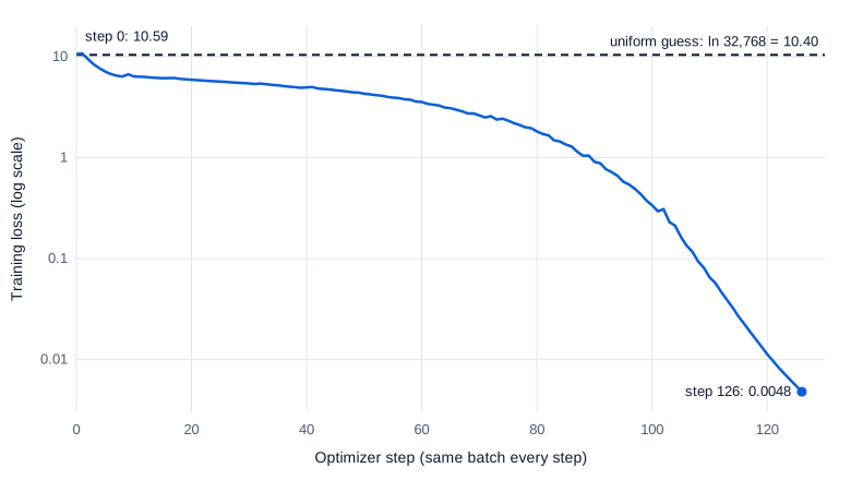
A model can pass all three checks and still not learn, if some tensor is detached from the graph or never reaches the optimizer. The standard test is to train on one fixed batch until it’s memorized: the 88M model, one batch of 4 × 1,024 held-out tokens, AdamW (Part 5 explains it) at a learning rate of 0.001 with no weight decay, gradient clipping at 1.0, BF16 autocast, seed 1337, no compilation. After the first backward pass, all 92 parameter tensors had nonzero gradients.
Swipe to pan the diagram, or tap it to zoom.
The loss fell from 10.59 to 0.0048 in 126 steps and about 30 seconds, after a brief spike at step 1. Given the batch’s first 16 tokens, “A continuation of our predictions of big issues for 2011…”, generate() with temperature=0 then wrote the next 48 tokens exactly as the document has them: “Don’t expect the debates on teaching quality to end anytime soon. We suspect that data from test scores (a la the Los Angeles Times series of 2010) will continue to be used to determine a teacher’s effectiveness in the”. Three runs of the same script took 119, 136 and 126 steps. Some GPU backward kernels add partial results in whatever order threads finish, so runs differ slightly even with a fixed seed.
Step 6: speed and memory against Part 1’s prototype
Part 1 timed a throwaway prototype of the same shape, and the real model should match it. Both were timed by one script in one session, alternating: forward and backward passes only, BF16 autocast, held-out text in 1,024-token sequences, after a warm-up of two micro-batches and one AdamW step (so optimizer memory counts), wall-clock time with torch.cuda.synchronize() on both sides, median of the timed micro-batches.
| Model and mode | Micro-batch | model.py: seconds (tokens/s) | Prototype: seconds (tokens/s) | Peak memory, model.py vs prototype |
|---|---|---|---|---|
| 88M, torch.compile, run 1 | 16 | 0.587 (27,915) | 0.592 (27,675) | 6.74 vs 6.81 GiB |
| 88M, torch.compile, run 2 | 16 | 0.599 (27,376) | 0.608 (26,959) | 6.74 vs 6.81 GiB |
| 22M, torch.compile | 16 | 0.174 (93,957) | 0.175 (93,485) | 2.68 vs 2.70 GiB |
| 88M, eager | 4 | 0.219 (18,708) | 0.198 (20,686) | 4.63 vs 4.34 GiB |
Hardware and software: NVIDIA GeForce RTX 4060 Laptop GPU (8 GB), driver 592.82, PyTorch 2.11.0 with CUDA 12.8, Triton 3.6.0. During the timed windows the median SM clock was 1,620 to 1,815 MHz, the memory clock held 7,000 MHz (one sample at 5,870), power averaged 38 to 42 W and the GPU ran at 66 to 75 °C. nvidia-smi -q reported a 40.5 W power limit right after the runs, below the 45 to 50 W during Part 1.
Compiled, model.py matches the prototype’s speed, uses slightly less memory, and peaks about 1.2 GiB below the card’s 8 GiB at 16 sequences. At 27,915 tokens per second and Part 1’s 622.95 million FLOPs per token, the forward and backward passes run at 17.4 TFLOPS, 69% of the GPU’s measured 25.3. The 22M model ran at about 94,000 tokens per second here against 102,400 in Part 1, but the prototype slowed by the same amount, so that’s today’s lower power limit, not the code.
In plain “eager” mode, without torch.compile, every operation runs as its own GPU kernel:
| 88M model, eager | Micro-batch 1 | Micro-batch 2 | Micro-batch 4 | Micro-batch 8 | Micro-batch 16 |
|---|---|---|---|---|---|
| Tokens/s | 15,411 | 18,812 | 18,708 | out of memory | out of memory |
| Peak memory | 2.28 GiB | 3.06 GiB | 4.63 GiB | n/a | n/a |
Eager mode needs about 0.78 GiB per sequence, against 0.33 GiB compiled. Measured inside one eager forward pass at 4 sequences, the ten blocks keep about 41 KB per token per layer for the backward pass, 1.7 GiB in all, and the loss briefly needs another 1.3 GiB for FP32 copies of 134 million logits. Compilation fuses the norm, RoPE, SwiGLU and loss arithmetic into kernels that never write those intermediates to memory, as GPU Part 9 measured on smaller examples. Eager model.py is also 10% slower than the eager prototype, most likely because its hand-written RMSNorm and FP32 RoPE each run as several small kernels; compiled, the difference disappears. Part 6 measures what compilation and its parts buy.
In the real world
The same decisions in published models:
| Model | RoPE pairs | Norm epsilon | Tied tables | Initialization |
|---|---|---|---|---|
| This series (88M) | Neighbors (2i, 2i+1), base 10,000 | 1e-5 | Yes | N(0, 0.02); residual outputs 0.02/√(2L) |
| Llama 3, Meta reference code | Neighbors, as complex numbers; base 500,000 | 1e-5 | No | Not in the released code |
Hugging Face LlamaForCausalLM | Halves (i, i + d_h/2) | Default 1e-6 | Default no | N(0, initializer_range), default 0.02 |
| SmolLM2-135M | Halves; base 100,000 | 1e-5 | Yes | Config’s initializer_range: 0.0417 |
| OLMo 2 1B | Halves; base 500,000 | 1e-6 | No | N(0, 0.02) for every parameter |
Sources: Meta’s Llama 3 model code and arguments (norm_eps: float = 1e-5, rope_theta: float = 500000); LlamaConfig and modeling_llama.py in transformers 5.20.2; the SmolLM2-135M config; the OLMo 2 1B config and the OLMo 2 paper.
- Meta’s RMSNorm is our line,
x * torch.rsqrt(x.pow(2).mean(-1, keepdim=True) + self.eps)applied tox.float(), and its RoPE views each neighboring pair as one complex number withtorch.view_as_complex. That’s why Hugging Face’s conversion script permutes the query and key weights. - SmolLM2-135M is the published model closest to ours: width 576, 30 layers, 9 query heads sharing 3 key-value heads, tied tables, the same epsilon. Its config records the layout as
"rope_interleaved": false, and itsinitializer_rangeof 0.0417 is exactly1/√576. Hugging Face uses that value for fresh models; how SmolLM2 initialized its own training isn’t in the checkpoint. - OLMo 2 dropped the residual scaling. Its paper says “we initialize every parameter from a normal distribution with a mean of 0 and a standard deviation of 0.02,” replacing a scheme in which “later layers were initialized to smaller values,” and shows the new one training more stably. For 10 layers either is reasonable; this series uses GPT-2’s because nanoGPT and llm.c, the closest public reference runs, both use it.
Common misconceptions
- “If the loss goes down, the model is correct.” The un-permuted RoPE model in Step 4 is a working Llama with scrambled positions, and it would train. A reference comparison catches that in seconds.
- “The starting loss should be exactly ln(vocabulary size).” Only if the logits start out equal. With GPT-2’s initialization they spread with a standard deviation of 0.554, which predicts 10.55. A big departure from the prediction is the warning sign.
- “Two Llama implementations are interchangeable.” They compute the same function, but Meta pairs RoPE numbers as neighbors and Hugging Face pairs the two halves of each head, and their default epsilons differ tenfold. Weights only move between them with a conversion.
- “The model code decides how much memory training needs.” The same 179 lines need 0.78 GiB per sequence in eager mode and 0.33 GiB compiled, and merely returning the logits from
forwardbroke the 16-sequence plan.
Key takeaways
- The series’ model is a Llama-style decoder in 179 lines of PyTorch: tied embeddings, RMSNorm, RoPE, grouped-query attention through PyTorch’s fused attention call, SwiGLU and pre-norm blocks, with 88,096,512 parameters, exactly what the formula says.
- Hugging Face’s Llama, given the same weights, matches our logits to 0.0003 in FP32, but only after reordering the query and key rows for its RoPE layout and matching the norm epsilon.
- The untrained model starts at a loss near 10.55, not 10.40, because the initialization gives the logits a spread of 0.554, and that gap can be worked out before running anything.
- Memorizing one batch, from 10.59 to 0.005 in 126 steps, and reproducing it word for word with
generate()shows that gradients reach every weight. - Compiled, the model is as fast as Part 1’s prototype, about 27,900 tokens per second, and fits 16 sequences in 6.74 GiB; uncompiled, it fits only 4.
What’s next
The model can learn one batch. Part 5 teaches it to learn from a billion tokens: the full training loop with AdamW, learning-rate warm-up and cosine decay, gradient clipping, BF16 and gradient accumulation, run first on the 22M model to draw the series’ first real loss curve.
Further reading
- RoFormer: Enhanced Transformer with Rotary Position Embedding (Su et al., 2021): RoPE, which “encodes the absolute position with a rotation matrix” while making attention depend on relative position.
- Using the Output Embedding to Improve Language Models (Press & Wolf, 2016): the case for tying the input and output embedding tables.
- Language Models are Unsupervised Multitask Learners (Radford et al., 2019): GPT-2, including the 1/√N scaling of residual layers at initialization.
- 2 OLMo 2 Furious (OLMo team, 2024): an open model’s account of its initialization and why it dropped residual scaling.
- Meta Llama 3 reference model code: RMSNorm, complex-number RoPE and grouped-query attention in about 300 lines.
- Hugging Face Llama conversion script: the
permutefunction that translates between the two RoPE layouts. - PyTorch
scaled_dot_product_attentiondocumentation:is_causal,enable_gqaand the reference math the fused kernels implement. - nanoGPT
model.py(Andrej Karpathy): a GPT-2 in one readable file, and the initialization this series copies.