
Inside the Model: Interpretability · Part 1 of 12
Opening the Black Box: What Interpretability Can Explain
What interpretability is for, its main methods, what counts as an explanation, and the toolkit, tested by asking two methods where GPT-2 keeps facts.
On this page
TL;DR
Interpretability studies what a trained model computes inside, and this series opens real models on a laptop to measure it. This first part covers what the field is for, its families of methods, and which of them show correlations and which test causes. It sets the bar for an explanation: faithful to the model, complete, minimal, and able to predict what happens when you change something. Then it builds the toolkit every later part uses, TransformerLens with its hooks and activation cache, and runs it on 168 landmark prompts, where two standard methods point at different parts of the same model.
Why it matters
Ask GPT-2 small to finish “The Eiffel Tower is located in the city of” and it says ” London”. Run it again without the start-of-text token that TransformerLens, the library used in this series, puts in front of every prompt by default, and it says ” Paris”. Fundamentals Part 16 fed the prompt without that token and got Paris. One invisible token flipped the answer, and nothing in the output tells you why.
Looking inside should tell you why, but “looking inside” covers many methods, and they don’t always agree. On 168 landmark prompts, we asked two of them which parts of GPT-2 small produce the right city. The score is in logits, the numbers a model gives each possible next token before turning them into probabilities. The first method credits the attention layers near the top of the model and gives the very first MLP, the two-layer network inside each block, 0.01 logits of credit. The second method removes that MLP and finds the model’s preference for the right city drops by 1.17 logits, more than for any other layer.
Both measurements are correct, because they answer different questions. This part shows how to tell those questions apart, and why the answer to the second one depends on how you remove a part.
The intuition
Think of a restaurant kitchen sending out one dish. You can ask “who put what on the plate?”: the sauce cook added the sauce, the grill cook the steak. Or you can ask “what happens if this cook stays home tonight?”
The answers differ. The prep cook who chops onions all afternoon never touches a plate, so the first question gives them no credit, yet without them half the dishes fail. And when the sauce cook is out, the grill cook may improvise a sauce, so the second question underrates the sauce cook. Direct attribution asks the first question. Ablation, which means removing a part and rerunning, asks the second.
The analogy breaks in two places. A model’s layers aren’t people with fixed jobs; every layer reads a blend of everything written before it. And a layer can’t simply “stay home”. Its output has to be replaced with something, zeros or an average, and as the experiment below shows, the choice changes the answer.
Step 1: what interpretability is for, and its methods
Interpretability research reads a model’s activations (the numbers it computes on the way to an output) and weights to work out how it behaves. Open Problems in Mechanistic Interpretability (Sharkey et al., 2025) describes the aim as understanding “the computational mechanisms underlying neural networks’ capabilities in order to accomplish concrete scientific and engineering goals.” Four goals come up again and again:
- Debugging: finding why a model fails on an input, such as the start token above, and whether a fix addresses the cause or a symptom.
- Safety: checking for behavior that outputs alone can hide. In a blind test, teams with access to a model’s internals found a hidden objective that a team with only API access missed.
- Science: learning how a network represents and combines knowledge, the way induction heads explained part of how models learn from their prompt.
- Control: changing behavior on purpose by editing internals, as steering vectors do by adding a direction to the activations while the model generates.
The methods fall into a few families, and the third column of the table carries the main distinction. A correlational method observes the model running normally and reports what is there or what was written. A causal method changes something inside and measures what happens to the output.
| Method | The question it answers | Kind of evidence | Where in this series |
|---|---|---|---|
| Behavioral tests | What does the model do on inputs built to probe a skill? | Outside view only | This part (the prompt set) |
| Direct attribution | How much did each part write toward the answer? | Correlational | This part, Part 2 |
| Probing | Can a simple classifier read a property from the activations? | Correlational | Part 3 |
| Ablation | What breaks when a part is removed? | Causal | This part, Part 4 |
| Activation patching | Which parts carry the difference between two inputs? | Causal | Part 5 |
| Features | What are the units the activations are built from? | Correlational, until tested | Parts 6 and 7 |
| Circuits | Which features and parts connect, step by step? | Both, tested by intervention | Parts 4 and 8 |
| Steering | Does adding a direction change behavior as predicted? | Causal | Part 9 |

Swipe to pan the diagram, or tap it to zoom.
Reading methods come first because they are cheap; the causal ones then test what the reading suggested.
Step 2: what counts as an explanation
A plausible story about a model is easy to write; showing that it describes what the model computes is harder. The paper that traced how GPT-2 small completes “When Mary and John went to the store, John gave a drink to” with “Mary”, Wang et al. (2022), turned that into three tests:
- Faithfulness: the circuit “can perform the task as well as the whole model”. Their 26-head circuit, run with everything else knocked out, “achieves 87% of the performance” of the full model, measured as the gap in logits between the right and wrong name.
- Completeness: the circuit “contains all the nodes used to perform the task”. Faithfulness alone can’t show this, because a model can carry two redundant copies of a mechanism and either one passes the first test.
- Minimality: the circuit “doesn’t contain nodes irrelevant to the task”.
The tests also found gaps: a greedy search found sets of heads whose removal affected the circuit and the full model differently by up to 87% of the original logit difference.
Current practice adds a fourth test: the explanation must predict what happens when you intervene. Anthropic’s attribution graphs (Part 8) explain a model through a simpler replacement model that matches the real model’s next-token completion on 50% of a diverse set of prompts, so every claim has to be checked on the real model. The authors call agreement under those checks “mechanistic faithfulness”, and the companion paper is explicit: “we regard the effects of interventions on the model’s actual outputs as the most important source of validation.” Even then, the attribution graphs gave “satisfying insight for about a quarter of the prompts” the team tried.
So a good explanation names parts, says what each one does, survives removing the parts it says don’t matter, and correctly predicts the effect of changing the parts it says do. Correlational evidence can suggest such a story. Only causal evidence can pass the last test.
Step 3: the toolkit, hooks and the activation cache
The residual stream, from Fundamentals Part 6, is the running vector per token that each attention layer and MLP reads from and adds its output to. A Mathematical Framework for Transformer Circuits (Elhage et al., 2021) describes it as a channel: the layers “communicate with each other by reading and writing to different subspaces of the residual stream.” Because every layer adds instead of overwriting, the final vector is exactly the sum of the token embedding, the position embedding and every layer’s output. That sum is what makes per-layer attribution possible.
TransformerLens, created by Neel Nanda and MIT-licensed, wraps open models so that every internal activation is exposed. Each activation passes through a hook point, a named spot such as blocks.9.hook_attn_out (the output of layer 9’s attention) where your own function can read or replace the value. run_with_cache runs the model once and keeps every activation in a dictionary called the activation cache. run_with_hooks runs it with your functions attached.
This listing runs as shown on GPU with TransformerLens 3.9.0, PyTorch 2.11 and GPT-2 small (124 million parameters, MIT license, Hugging Face ID openai-community/gpt2) in fp32 (32-bit floats):
import torch
from transformer_lens import HookedTransformer

torch.set_grad_enabled(False)
model = HookedTransformer.from_pretrained("gpt2", device="cuda")  # fp32, LayerNorm folded
prompt = "The Brandenburg Gate is located in the city of"
logits, cache = model.run_with_cache(prompt)
print(model.to_str_tokens(prompt))
print(len(cache), "cached activations;", cache["blocks.9.hook_attn_out"].shape)
print("top guess:", model.to_string(logits[0, -1].argmax()))

# Direct logit attribution: what each piece writes toward " Berlin" rather than " Munich"
ans, alt = model.to_single_token(" Berlin"), model.to_single_token(" Munich")
direction = model.W_U[:, ans] - model.W_U[:, alt]
parts, labels = cache.decompose_resid(layer=-1, apply_ln=True, pos_slice=-1, return_labels=True)
dla = parts[:, 0] @ direction
for i in dla.abs().argsort(descending=True)[:4]:
    print(f"{labels[i]:>8}  {dla[i]:+.2f}")
print("logit diff:", round((logits[0, -1, ans] - logits[0, -1, alt]).item(), 2))

# Ablation: zero MLP 0's output at every position after <|endoftext|>, rerun
def zero_mlp0(act, hook):
    act[:, 1:] = 0
    return act

ablated = model.run_with_hooks(prompt, fwd_hooks=[("blocks.0.hook_mlp_out", zero_mlp0)])
print("ablated logit diff:", round((ablated[0, -1, ans] - ablated[0, -1, alt]).item(), 2))
print("ablated top guess:", model.to_string(ablated[0, -1].argmax()))
It prints (TransformerLens 3.9 also warns on stderr that from_pretrained is deprecated):
Loaded pretrained model gpt2 into HookedTransformer
['<|endoftext|>', 'The', ' Brand', 'enburg', ' Gate', ' is', ' located', ' in', ' the', ' city', ' of']
210 cached activations; torch.Size([1, 11, 768])
top guess:  Berlin
11_mlp_out  -0.78
8_attn_out  +0.73
10_attn_out  +0.53
11_attn_out  +0.47
logit diff: 1.75
ablated logit diff: 2.27
ablated top guess:  the
from_pretrained applies weight processing by default: it folds each LayerNorm’s learned scale into the next weight matrix and centers the weights that write to the residual stream. The outputs don’t change, but “the residual stream” now means the centered version, and so does any direction in it. from_pretrained_no_processing keeps the Hugging Face weights unchanged, and each part says which it used. TransformerLens 4.0 replaces this API with TransformerBridge; the ideas carry over.
The cache holds 210 named activations; blocks.9.hook_attn_out alone is one 768-number vector for each of the 11 tokens. Direct logit attribution (DLA) is the dot product in the middle of the listing. decompose_resid splits the final residual stream into its pieces and scales each one by the final LayerNorm, using the scale from this exact run, and the dot product with the unembedding direction for ” Berlin” minus ” Munich” turns each piece into logits. The pieces add up to the model’s logit difference, so DLA says how much each piece wrote toward the answer: here attention layers 8, 10 and 11 push toward Berlin and MLP 11 pushes back. It doesn’t say how a piece got its input.
Ablation is the last block: a hook that overwrites MLP 0’s output, then a rerun. It zeroes every position after the start token, which is the same in every prompt and is left alone throughout this article. The result is a warning about metrics. Zeroing MLP 0 widens the Berlin-over-Munich gap from 1.75 to 2.27 logits, yet the model stops naming a city at all: its top guess becomes ” the”. A score that compares two answers can’t see damage that hits both, which is why the experiment below also reports accuracy. Zeroing is also the bluntest kind of ablation. Mean ablation replaces the output with its average over the prompt set instead, removing only what varies from prompt to prompt.
Step 4: one behavior, three ways
The behavior is factual recall: completing “[landmark] is located in the city of” with the right city.
The prompt set was built by hand for this article: 168 landmarks in 54 cities, from “The Brandenburg Gate” (Berlin) to “Graceland” (Memphis). The rules were that no landmark name contains its city, the landmark sits inside the city proper, ambiguous names were dropped (there is a Pantheon in both Rome and Paris), and every city is a single token for both models used here. GPT-2 runs in fp32 with weight processing on, on an NVIDIA GeForce RTX 4060 Laptop GPU (8 GB).
The score for each prompt is the logit difference between the right city and the average of the other 53 cities. It adds up exactly across the pieces of the residual stream: the sum of all DLA terms plus the output bias matched the model’s logit difference to within 0.00002 logits on every prompt. Every interval below is a 95% bootstrap confidence interval over the 168 prompts (10,000 resamples), or a Wilson interval for accuracies.
| GPT-2 small on 168 landmark prompts | Result |
|---|---|
| Right city is the top token out of 50,257 | 14.9% (10.3 to 21.0%) |
| Right city ranks first among the 54 cities | 39.9% (32.8 to 47.4%); chance is 1.9% |
| Mean logit difference, right city vs the others | 3.57 (3.17 to 3.97) |
GPT-2 small is a weak fact-recaller. On the prompts it misses, its top token is often the first letter of the landmark (” T” for “Tiananmen Square”) or a big city like ” London”. But a logit difference of 3.57 means the right city is, on average, about 35 times more likely than a typical wrong one (e to the power 3.57), a signal big enough to trace.
Method 1: direct logit attribution
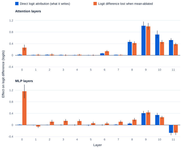
DLA splits the 3.57 logits across the 26 pieces of the residual stream at the last token: the two embeddings and 12 attention and 12 MLP outputs. The answer is concentrated near the top of the model. Attention layer 9 writes +1.02 logits (0.88 to 1.16), layer 10 +0.72, layer 11 +0.52 and layer 8 +0.46. MLPs 9 and 10 add +0.41 and +0.35. MLP 11 writes against the answer, at -0.27 (-0.35 to -0.19). Every layer from 0 to 7 writes less than 0.07 logits either way.
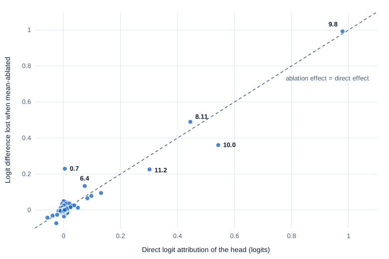
Split further by attention head, one head stands out: head 9.8 (layer 9, head 8) writes +0.98 logits (0.85 to 1.11) on its own, almost all of its layer’s total. Heads 10.0, 8.11 and 11.2 add +0.54, +0.44 and +0.30.
Read alone, DLA tells a tidy story: late attention heads copy the city into the last position, much as Geva et al. (2023) describe attention heads extracting an attribute from the subject in GPT-2 XL and GPT-J. DLA is correlational, though: it reports what was written and says nothing about what was needed.
Method 2: ablation
Ablation removes each of the 24 layer outputs in turn, at every position after the start token, and measures the change in logit difference. Mean ablation uses one average per position of the template (” is”, ” located”, …, ” of”) and one for the landmark’s tokens, following the IOI paper’s practice of averaging per template position. Zero ablation sets the output to 0.
Swipe to pan the diagram, or tap it to zoom.
For the late attention layers, the two methods agree. Mean-ablating attention layer 9 costs 1.00 logits (0.88 to 1.12), almost exactly its DLA of 1.02. The same holds for head 9.8: ablating it costs 0.99 logits.
The biggest single effect, though, is a layer DLA ignored. Mean-ablating MLP 0 costs 1.17 logits (0.92 to 1.40), more than any other layer. On the 67 prompts where GPT-2 ranked the right city first, it now does so on only 57% of them. MLPs 2 to 8, also invisible to DLA, each cost between 0.05 and 0.18 logits. These early MLPs write nothing toward the city directly; they build up a representation of the landmark that later layers read, which fits the “subject enrichment” by early MLPs in Geva et al.
Method 3: measuring the disagreement
The two methods can be compared on the same scale. If a layer’s only influence on the answer were its direct write, mean-ablating it would cost exactly its DLA minus the DLA of its mean, the direct effect. Whatever is left over is the indirect effect: the change that flows through later layers.
| Layer | DLA (logits) | Lost when mean-ablated | Direct part | Indirect part | Lost when zero-ablated |
|---|---|---|---|---|---|
| MLP 0 | +0.01 | 1.17 (0.92 to 1.40) | 0.00 | 1.17 | 2.01 |
| Attention 0 | +0.02 | 0.27 (0.17 to 0.37) | 0.02 | 0.25 | 2.78 |
| Attention 9 | +1.02 | 1.00 (0.88 to 1.12) | 1.00 | 0.00 | 0.90 |
| Attention 10 | +0.72 | 0.46 (0.39 to 0.53) | 0.70 | -0.24 | 0.38 |
| MLP 9 | +0.41 | 0.43 (0.36 to 0.51) | 0.39 | 0.05 | -0.20 |
| MLP 11 | -0.27 | -0.26 (-0.34 to -0.19) | -0.25 | -0.02 | -1.14 |
Some layers matter only indirectly. MLP 0’s whole effect is indirect, and so is almost all of attention layer 0’s. A single head shows it too: head 0.7 writes +0.005 logits toward the answer, yet ablating it costs 0.23 logits (0.14 to 0.32).
Some layers are partly replaced when removed. Attention layer 10 writes 0.72 logits, but removing it costs only 0.46; the other 0.24 logits come back from later layers that change their output when layer 10 goes quiet. McGrath et al. (2023) named this compensation the Hydra effect in Chinchilla 7B, and also found “late MLP layers that act to downregulate the maximum-likelihood token”. GPT-2’s MLP 11 behaves that way here: it pushes against the answer, and removing it helps.
Zero ablation tells a third story. Zeroing attention layer 0 costs 2.78 logits, ten times what mean-ablating it costs, and leaves the right city first among the 54 on only 11.9% of prompts. Zeroing MLPs 9 and 10 even raises the logit difference, by 0.20 and 0.21. Zero is a value these layers never output, so later layers get inputs unlike anything seen in training; the IOI authors call 0 “an arbitrary value” and found zero ablation “to lead to noisy results in practice.”
Across all 24 layer outputs, the rank correlation between DLA and the mean-ablation cost is 0.69 (0.54 to 0.81). Between DLA and the zero-ablation cost it falls to 0.37 (0.21 to 0.48). The direct parts add up to 67% (61 to 73%) of the total absolute mean-ablation effect, so a third of what the layers do to the answer runs through other layers.
Swipe to pan the diagram, or tap it to zoom.
Heads on the diagonal act directly, heads above it work through other parts, and heads below it are partly replaced when they’re removed.
The causal number also depends on how the average is taken. Computing a single average over all positions, instead of one per template position, moves MLP 9’s ablation cost from 0.43 to 0.07 logits and MLP 0’s from 1.17 to 1.62. “What the model needs” depends on what you replace a part with, which is why Part 5 replaces it with activations from a real alternative prompt instead.
Does it carry over to a modern model?
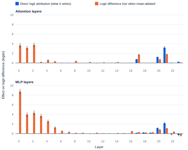
Qwen2.5-0.5B (494 million parameters, Apache-2.0, Qwen/Qwen2.5-0.5B) is a 2024 model with 24 layers. It was loaded with from_pretrained_no_processing, its bf16 weights upcast to fp32, and DLA applies its final RMSNorm scale and gain explicitly; the pieces again summed to the logit difference within 0.00003 logits. Qwen has no start token, so each prompt’s first token, usually “The”, was left unablated. It knows the landmarks far better: the right city is its top token on 66.1% of prompts (58.6 to 72.8%), first among the 54 cities on 82.7% (76.3 to 87.7%), with a mean logit difference of 9.27 (8.73 to 9.81).
Swipe to pan the diagram, or tap it to zoom.
The pattern from GPT-2 holds and gets stronger. DLA puts the answer in layers 17 to 21: attention layer 21 writes +3.20 logits (2.89 to 3.51) and MLP 21 +2.18. Mean ablation puts the largest costs at the bottom. Removing MLP 0 costs 8.73 logits (8.16 to 9.31), nearly the whole logit difference, and leaves the right city first on only 4% of prompts. At the top, repair is stronger too: removing attention layer 21 costs 1.80 of the 3.20 logits it writes, so 1.38 logits come back from the layers after it.
| Agreement between DLA and mean ablation, over all layer outputs | GPT-2 small | Qwen2.5-0.5B |
|---|---|---|
| Rank correlation | 0.69 (0.54 to 0.81) | 0.16 (0.03 to 0.26) |
| Layers in both top-5 lists | 4 of 5 | 0 of 5 |
| Direct part of the total ablation effect | 67% (61 to 73%) | 21% (19 to 23%) |
On Qwen, attribution alone would send you to the wrong half of the network. A caution applies to both models, though. Early layers run on every token, so removing one damages every word’s representation, not just the landmark’s. A large early-layer cost says the answer depends on that layer, not that the fact is stored there. Telling those apart takes the controlled swaps of Part 5.
In the real world
These patterns show up in the literature at larger scale, though none of the following was reproduced here.
The IOI circuit in GPT-2 small (Wang et al., 2022) is 26 attention heads in 7 classes, 1.1% of the model’s (head, position) pairs. Its backup name-mover heads are the Hydra effect in miniature: knock out the main name movers and other heads take over. The authors mean-ablated over prompts with three unrelated names, because averaging over the task’s own prompts “would not remove enough information helpful for the task”. The landmark experiment averaged over its own prompts, so its mean ablations leave in place whatever all of them share, such as “a city name comes next”.
Geva et al. (2023) studied factual recall in GPT-2 XL (48 layers, 1.5 billion parameters) and GPT-J (28 layers) with interventions. They describe three steps: early MLPs enrich the subject’s last token with attributes, the relation’s information moves to the last position, and attention heads there extract the attribute.
McGrath et al. (2023) saw later layers of Chinchilla 7B raise their own direct effect when one attention layer was ablated, “even in language models trained without any form of dropout”, the training trick that randomly switches parts off. So a small ablation effect never proves a part is unimportant.
On frontier models the split between reading and intervening still holds. Anthropic’s 2025 study of Claude 3.5 Haiku read a Dallas-to-Texas-to-Austin path off an attribution graph, then confirmed it by intervening: swapping in “California” features changed the answer from “Austin” to “Sacramento” (Lindsey et al., 2025; not reproduced here).
Common misconceptions
- “If a component writes the answer, that’s where the knowledge lives.” DLA shows only the last step. GPT-2’s head 9.8 writes the city, but MLP 0, which writes nothing toward it, costs more when removed.
- “Removing a part shows exactly how much it matters.” It shows what is lost after the rest of the network adapts. Attention layer 10 writes 0.72 logits but costs only 0.46 when removed.
- “Zero ablation is the neutral way to turn something off.” Zero is a value most layers never produce. Zeroing GPT-2’s attention layer 0 costs ten times what mean-ablating it does, and zeroing MLPs 9 and 10 flips the sign of their effect.
- “A correlation inside the model is an explanation.” A probe, an attention pattern or an attribution shows what is present or written. An explanation also has to predict what interventions do, the test both the IOI paper and Anthropic’s 2025 work treat as decisive.
- “One famous prompt is enough to show a mechanism.” The Eiffel Tower prompt flips between London and Paris on the start token alone. Results need a prompt set, an interval, and a check that they hold up when the setup changes.
Key takeaways
- Interpretability has four goals, debugging, safety, science and control, and two kinds of evidence: correlational methods read what is there, causal methods change something and watch.
- A good explanation is faithful, complete and minimal, and it predicts what interventions will do; the IOI circuit reached 87% faithfulness and still showed gaps in completeness.
- TransformerLens exposes every activation through hooks and an activation cache. Because the residual stream is a sum, direct logit attribution splits GPT-2’s answer exactly across its layers.
- On 168 landmark prompts, attribution and mean ablation agree on GPT-2’s late heads that write the city, with head 9.8 at about 1 logit by both, but only ablation finds that MLP 0 matters most. On Qwen2.5-0.5B the two methods barely agree at all, with a rank correlation of 0.16.
- The causal number depends on the ablation: zeroing and averaging can differ tenfold or flip sign, and later layers partly repair what you remove.
What’s next
DLA read only the very top of the residual stream. Part 2 reads it at every layer, turning half-finished vectors into words with the logit lens, and shows where that simple trick fails and how a trained “tuned lens” fixes it.
Further reading
- Interpretability in the Wild: a Circuit for Indirect Object Identification in GPT-2 small (Wang et al., 2022): the faithfulness, completeness and minimality tests, and why mean ablation beats zero ablation.
- Circuit Tracing: Revealing Computational Graphs in Language Models (Ameisen et al., 2025): replacement models, error nodes and mechanistic faithfulness.
- On the Biology of a Large Language Model (Lindsey et al., 2025): case studies in Claude 3.5 Haiku, each validated by intervention.
- The Hydra Effect: Emergent Self-repair in Language Model Computations (McGrath et al., 2023): why ablation effects underrate a part, and late MLPs that push back on the top token.
- Dissecting Recall of Factual Associations in Auto-Regressive Language Models (Geva et al., 2023): subject enrichment and attribute extraction in GPT-2 XL and GPT-J.
- A Mathematical Framework for Transformer Circuits (Elhage et al., 2021): the residual stream as a channel, and why outputs decompose into paths.
- Open Problems in Mechanistic Interpretability (Sharkey et al., 2025): the field’s goals and what it can’t do yet.
- How to use and interpret activation patching (Heimersheim & Nanda, 2024): practical advice on interventions, metrics and their pitfalls.
- TransformerLens (GitHub): the library used throughout this series.
- Inside the Black Box: Features, Superposition and Circuits (Fundamentals Part 16): the one-article overview of the whole field.