
Build an LLM From Scratch · Part 7 of 15
Build an LLM From Scratch: The Pretraining Run
16.8 hours, 1.76 billion tokens, 0.83 kWh: the 88M model's run on a laptop GPU, read through its loss curves, spikes, held-out loss and samples.
On this page
TL;DR
The series’ 88M-parameter model trained on 1.76 billion FineWeb-Edu tokens in 16 hours 49 minutes on the laptop’s RTX 4060, in one try, with no crash and no resume. Training steps ran at 29,399 tokens per second, within 0.03% of Part 6’s prediction, and the GPU used 0.83 kWh. Validation loss fell from 10.59 to 3.38. Half of that drop came in the first 1.5% of the tokens; the last 30% of the run bought 0.07. On the whole held-out shard the final loss is 3.365, 1.61 lower than Part 5’s 22M model. The gradient norm went above the clipping threshold only 12 times after warm-up, all before step 495, and the biggest jumps in the training loss came from hard batches. Samples from 49 saved snapshots show the model going from one repeated word, to “the the the”, to fluent English with invented facts.
Why it matters
At step 25 of this run, the model wrote the same text no matter what you asked it. Three different prompts, sampled with the same random seed, came back as near-identical strings of “the”, “of” and commas. By step 3,360 it continues “In 1492, Christopher Columbus” with “first sailed from the New World.” It also says he sailed “from New York to New York.”
Everything between those two outputs happened unattended, overnight. A 17-hour run can’t be watched, only read afterwards from what it wrote down: a log line per step, a validation loss every 50 steps, a power reading every second, and 49 copies of the weights. This part reads them, and checks three promises: Part 6’s 16.6 hours of training steps, Part 1’s 0.8 kWh, and Part 5’s plan to watch the embedding’s norm.
The intuition
Think of a long-haul flight on autopilot. Nobody steers, but the flight recorder logs altitude, speed and engine heat every second. A smooth flight and a flight that nearly stalled can land at the same airport; only the recorder tells them apart.
The training log is that recorder. The loss is the altitude on the descent: it should drop fast, then level out. The gradient norm, the size of each step’s correction, is turbulence: a jolt shows there first. The validation loss, measured on text the model never trains on, is a second instrument that checks the first.
The analogy breaks in one place. A plane’s turbulence comes from outside. A model’s jolts can come from the data, the optimizer or both, and the log alone can’t always say which; the saved weights can.
Step 1: the run, as launched
The command, run from the shared code folder under the GPU lock, with nvidia-smi logging clocks and power every second:
python train.py --model main --out runs/main88 --steps 3360 --warmup 150 --lr 6e-4 \
    --val-every 50 --ckpt-every 100 --keep-ckpts \
    --snapshot-at 0,5,10,15,20,25,30,40,50,60,75,90,125,150,250 \
    --compile --fused --resume
Two things differ from Part 5’s published command. Validation runs every 50 steps instead of 100, for a denser held-out curve, at a cost of about 4 minutes. And --snapshot-at is new: it saves extra weights-only snapshots at chosen steps, because most of the learning happens in the first few hundred steps, which a snapshot every 100 steps would barely see. --resume on a fresh run starts at step 0; it lets the wrapper script rerun the same command after a crash, which it never had to. The new option is three small additions to train.py:
# train.py (excerpts): the --snapshot-at option added for Part 7
p.add_argument("--snapshot-at", default="", help="extra steps for model-only snapshots, e.g. 0,10,25 (Part 7)")

snapshot_at = {int(s) for s in a.snapshot_at.split(",") if s}
if step == 0 and 0 in snapshot_at:                       # the untrained weights
    torch.save(raw.state_dict(), os.path.join(a.out, "model_00000.pt"))

        if step % a.ckpt_every == 0 or step == stop:      # in the loop, after each optimizer step
            save_checkpoint(ckpt_path, raw, opt, step, a)
            if a.keep_ckpts:
                torch.save(raw.state_dict(), os.path.join(a.out, f"model_{step:05d}.pt"))
        elif step in snapshot_at:
            torch.save(raw.state_dict(), os.path.join(a.out, f"model_{step:05d}.pt"))
A snapshot is the FP32 weights alone, 352 MB; a checkpoint adds AdamW’s state, 1.06 GB, for resuming. The run left 49 snapshots and 18 GB in its folder.
| Setting or result | Value |
|---|---|
| Model | 88,096,512 parameters: width 768, 10 layers, 12 query and 4 key-value heads, SwiGLU width 2,048, tied 32,768-token embedding |
| Data | 1,761,607,680 FineWeb-Edu tokens (Part 3’s shards), each seen once: 20.0 per parameter |
| Batch and steps | 524,288 tokens per step (16 sequences × 1,024 tokens × 32 micro-batches), 3,360 steps |
| Learning rate | 150 warm-up steps (78.6M tokens) to 6 × 10⁻⁴, cosine to 6 × 10⁻⁵ at step 3,360 |
| Optimizer | AdamW, betas (0.9, 0.95), epsilon 10⁻⁸, weight decay 0.1 on all matrices including the tied embedding, clipping at 1.0 |
| Precision and flags | BF16 autocast over FP32 weights; --compile --fused; seed 1337 |
| Hardware and software | NVIDIA GeForce RTX 4060 Laptop GPU (8 GB), WSL2, driver 592.82, PyTorch 2.11.0 with CUDA 12.8 |
| Wall time | 18:23 to 11:12 the next day: 16 h 49 min (60,544 s); not resumed |
| Throughput | 29,399 tokens/s over training steps, 29,101 over the whole job; MFU 72.4% |
| Peak GPU memory | 6.76 GiB |
| Validation loss | 10.59 at step 0, 6.93 at step 50, 4.19 at 500, 3.76 at 1,000, 3.50 at 2,000, 3.38 at 3,360 (40 micro-batches) |
| Energy at the GPU | 0.834 kWh, mean draw 49.6 W |
Step 2: 16.8 hours on a laptop
Where the time went
Each log line records its step’s duration, so the job’s 60,534 seconds split cleanly:
| Part of the job | Time | Share |
|---|---|---|
| 3,360 training steps | 59,920 s (16.64 h) | 99.0% |
| 69 validation passes, about 7 s each | about 8 min | 0.8% |
| 34 checkpoints and 49 snapshots | about 2 min | 0.2% |
| Compilation | a few seconds | under 0.1% |
Compilation nearly vanished because Inductor’s on-disk cache was warm from Part 6: step 0 took 19.1 seconds against a median of 18.4. Python’s start-up took the other 10 seconds of wall-clock time.
Throughput against the predictions
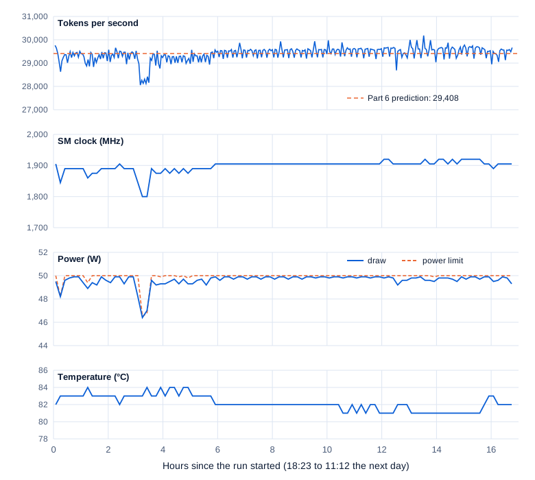
Part 6 measured 29,408 tokens per second over 32 steps and predicted 16.6 hours of training steps. The run’s steps averaged 29,399 tokens per second (total tokens over total step time) and took 16.64 hours. MFU (model FLOPs utilization) counts 622.95 million FLOPs per token against the 25.3 TFLOPS this GPU reached in GPU Part 4: 72.4% over the steps, 71.7% over the whole job. Part 1’s more cautious plan, at a sustained 28,296 tokens per second, said to allow about 18 hours. The job took 16.8.
Single steps were noisier. Their throughput alternated between about 27,000 and 31,000 tokens per second, a slow step almost always followed by a fast one (correlation between neighbouring step times −0.86), while the SM clock barely moved with it (correlation 0.11). So it looks like a timing artifact; the cause wasn’t traced. Over blocks of 10 steps, 90% ran between 28,952 and 29,685 tokens per second.
Swipe to pan the diagram, or tap it to zoom.
The one visible dip came about 3.2 hours in: the laptop lowered its power limit to about 46.5 W for 20 minutes, the clock fell from 1,890 to 1,800 MHz, and throughput fell 4%. After midnight the GPU ran a degree or two cooler and 15 MHz faster, and throughput rose about 1%.
Over all 56,877 one-second readings, the SM clock’s median was 1,905 MHz (90% between 1,740 and 1,935), and the memory clock held 7,000 MHz in all but 58. The power limit sat at exactly 50 W in 82% of readings, never below 42 W. The GPU ran at a median of 82 °C (81 to 84 °C for 90% of the run, maximum 85). In 99.8% of readings the only throttle reason was the software power cap: the GPU spent the whole run pushing against 50 W.
Integrating the power readings gives 0.834 kWh at the GPU board, against Part 1’s estimate of 0.8 (0.82 before rounding): 17 cents at an illustrative 20 cents per kWh. The rest of the laptop wasn’t measured.
Step 3: reading the loss curve
Swipe to pan the diagram, or tap it to zoom.
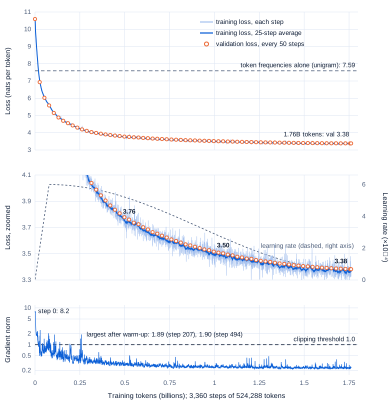
The three panels share one axis, so a jolt in the gradient norm lines up with the loss above it.
A fast drop, then a long tail
The loss is cross-entropy in nats per token (Math Part 6): how surprised the model is, on average, by each next token. At step 0 it’s 10.59, a little above ln 32,768 = 10.40, the score of a model that spreads its bets evenly over the vocabulary.
The dashed line at 7.59 is the unigram level, the entropy of the validation tokens’ own frequencies (recomputed here: 7.590 nats): what a model that knew only how often each token occurs would score. The training loss passed it at step 36, after 19 million tokens. Everything below comes from context.
Then the curve bends hard. Measured as a share of the whole drop from 10.59 to 3.38:
| Validation loss reached | Step | Tokens | Share of the run’s tokens | Share of the total drop |
|---|---|---|---|---|
| 6.93 | 50 | 26M | 1.5% | 51% |
| 4.88 | 250 | 131M | 7.4% | 79% |
| 4.19 | 500 | 262M | 14.9% | 89% |
| 3.76 | 1,000 | 524M | 29.8% | 95% |
| 3.38 | 3,360 | 1,762M | 100% | 100% |
Each successive 500 steps bought less: 6.40, then 0.43, 0.16, 0.094, 0.066, 0.040, and 0.015 over the last 360 steps. That shape, steep and then ever flatter, is roughly a power law in the tokens seen, the relationship Fundamentals Part 12 describes and Part 8 fits across model sizes.
The cosine in the last third
Over the last third the learning rate falls from 2.1 × 10⁻⁴ to its floor of 6 × 10⁻⁵, and the loss’s progress falls with it: 0.036 per 100 steps around step 1,000, 0.015 around step 2,000, 0.0055 around step 3,000, 0.0037 over the last 100. Near the floor each update is a tenth of its peak size, and the curve goes almost flat.
How much of the last third’s gain came from the decay itself, this run can’t show. A power law fitted to the validation curve over steps 300 to 2,240 predicts 3.386 at the end, against the 3.382 reached; fitted over steps 500 to 1,680 it predicts 3.401. So the decay’s bonus is between nothing and 0.02, depending on the fit. Separating it takes a second run at a constant rate, as Hägele et al. (2024) did: with a constant rate and a short final decay, “the sudden drop in loss” lined up with the decay.
Why validation sits on top of training
In a single pass over fresh data, every training batch is unseen text, and its loss is measured before the update that learns from it. So the training loss is itself a held-out measurement, and there’s nothing to overfit. From step 200 on, the validation loss sat 0.015 above the average training loss of the surrounding 10 steps (standard deviation 0.016). Even that is about which text was measured: the 655,360 tokens train.py checks are slightly harder than the validation shard as a whole.
Held-out loss on the whole shard
train.py’s 40 micro-batches are a fixed 4% sample of the validation shard. All 915 take 4.6 minutes per model (SM clock median about 2,000 MHz, 49 W), so they ran after training, on three snapshots, through a small new module, snapshots.py, that loads saved weights:
| Weights | Validation loss, 40-batch subset (655,360 tokens) | Validation loss, whole shard (14,991,360 tokens) | Difference |
|---|---|---|---|
| Step 1,000 | 3.7602 | 3.7438 | −0.0164 |
| Step 2,000 | 3.5029 | 3.4859 | −0.0170 |
| Step 3,360 (final) | 3.3823 | 3.3651 | −0.0172 |
| Part 5’s 22M model, final | 4.9657 | 4.9725 | +0.0068 |
The subset is a steady 0.017 harder than the whole shard, so the chart’s curve is shifted by a constant. The 88M model ends 1.61 below Part 5’s 22M model, with 4 times the parameters and 7.6 times the tokens. At equal tokens it was already ahead: 4.30 at step 450 (236 million tokens), against the 22M model’s 4.97 at the end of its 230.7-million-token run. Splitting the gap into size and tokens is Part 8’s job; what 3.37 means in bits per byte and on benchmarks is Part 9’s.
Step 4: spikes, noise and a referee
The gradient norm
The gradient norm is the length of the whole gradient, all 92 parameter tensors treated as one vector, measured before clipping scales it down to 1.0 (Part 5 explains the clip). In this run 72 steps were clipped. Sixty of them came during the 150 warm-up steps, while the learning rate was still small: the norm started at 8.2 for the untrained model, fell below 2.6 by step 8, and touched 2.51 at step 54 and 2.05 at step 143. After warm-up there were 12:
| Step | 151 | 154 | 160 | 161 | 167 | 195 | 207 | 221 | 263 | 370 | 483 | 494 |
|---|---|---|---|---|---|---|---|---|---|---|---|---|
| Norm before clipping | 1.25 | 1.43 | 1.13 | 1.04 | 1.01 | 1.17 | 1.89 | 1.23 | 1.19 | 1.06 | 1.46 | 1.90 |
None came after step 494. The median norm fell from 0.59 around step 150 to 0.29 around step 1,000 and 0.24 at the end, and after step 1,000 it never exceeded 0.52. The worst clip after warm-up scaled a gradient to 53% of its length. Part 5’s 22M run, with a 20-step warm-up and a peak rate 2.5 times higher, hit 30.8 at step 12; nothing like that happened here.
The loss barely noticed. Around step 207 it read 5.17, 5.13, 5.20, 5.13, 5.16 for steps 205 to 209, within the step-to-step noise of that phase. Around step 494 it read 4.17, 4.16, then 4.34 at step 495, then 4.25, 4.18. That step-495 jump looks like a spike’s aftermath, since the loss is measured before each update and step 494’s clipped update had just been applied.
Noise versus spikes
A loss spike is a rise caused by the model: an update overshoots and damages what it had learned, so the loss stays up or diverges. Batch noise is a rise caused by the text, because some batches are harder than others. Both look like a jump in the training loss.
Subtracting a 21-step moving average leaves the step-to-step noise: a standard deviation of 0.036, the same in each third of the run while the learning rate fell tenfold, a first clue that it’s mostly the data. The largest jump of the run, 0.20 above the local average, came at step 1,004, with an ordinary gradient norm of 0.45.
The saved weights can referee. Each training batch is a pure function of its step number (Part 3’s loader), so the same batches can be scored by snapshots from before and after:
| Loss of the training batch at step | 1,002 | 1,003 | 1,004 | 1,005 | 1,006 |
|---|---|---|---|---|---|
| Scored by the step-1,000 weights | 3.732 | 3.711 | 3.945 | 3.749 | 3.713 |
| Scored by the step-1,100 weights | 3.609 | 3.580 | 3.783 | 3.622 | 3.582 |
| Loss of the training batch at step | 493 | 494 | 495 | 496 | 497 |
|---|---|---|---|---|---|
| Scored by the step-400 weights | 4.394 | 4.396 | 4.552 | 4.471 | 4.411 |
| Scored by the step-500 weights | 4.004 | 4.060 | 4.169 | 4.104 | 4.064 |
Batch 1,004 is about 0.2 harder than its neighbours for weights that never saw it and for weights that trained past it: it’s the text. Batch 495 is 0.11 to 0.16 harder than batch 494 for both snapshots, which accounts for most of the 0.17 jump in training. The validation curve agrees: it fell 0.124, 0.104 and 0.083 over the 50-step windows ending at steps 450, 500 and 550, with no hiccup. This run had noise and clipped gradients, but no loss spikes.
Step 5: what the model writes, step by step
snapshots.py’s complete encodes a prompt with Part 2’s tokenizer and calls model.generate from Part 4 (no KV cache, so each new token reruns the whole prompt, which is fine at this size). Greedy decoding picks the most likely token every time; sampling here uses temperature 0.8 and top-k 50 with seed 0 (Fundamentals Part 9 explains both). Run from the folder that holds runs/main88:
from snapshots import load, complete

for step in (0, 25, 100, 250, 500, 1000, 2000, 3360):
    model = load(f"runs/main88/model_{step:05d}.pt")
    print(step, "greedy: ", complete(model, "The water cycle is", n_tokens=48))
    print(step, "sampled:", complete(model, "The water cycle is", n_tokens=48, temperature=0.8, top_k=50, seed=0))
Part 5’s 22M model, greedy, continued this prompt with “a major part of the water. The water is a major part of the water.” The 88M model’s greedy continuations, trimmed:
| Step | Validation loss | “The water cycle is”, greedy |
|---|---|---|
| 0 | 10.59 | description description description description description … |
| 25 | 8.30 (training) | , the the the the the the the the the the … |
| 100 | 6.03 | a few of the most of the most of the world, the most of the world, and the most of the world … |
| 250 | 4.88 | the most important part of the water supply chain. The water is the most important factor in the water supply chain. |
| 500 | 4.19 | the water cycle. The water cycle is the water cycle. The water cycle is the water cycle. |
| 1,000 | 3.76 | a very important factor in the water cycle. The water cycle is a very important factor in the water cycle. |
| 2,000 | 3.50 | the result of the natural flow of water through the earth’s surface. The water cycle is the result of the natural flow of water through the earth’s surface. |
| 3,360 | 3.38 | a complex process that requires a lot of energy and energy. The energy that is generated is stored in the water cycle, which is the water cycle. |
Greedy decoding loops at every stage: once a phrase is its own most likely continuation, it repeats. What changes is what loops: one random token at step 0, the most frequent word at step 25, phrases at step 100, sentences by step 250, a roughly true sentence at step 2,000.
Step 25’s sampled continuations for three different prompts were nearly identical, ” of the a the the of. The the the the, the the the the 2 to the the the,” for the water cycle and ” the. a the the of. The the the the, the, the the 2 to the the the,” for “The best way to learn a new language is”: with the same seed and a model that ignores its prompt, the same random draws give the same text. By step 1,000 the water cycle is “very important to the future of the Earth, and it is not a very important element for the earth, but it is a key component of life.”
Facts arrive last, and wrong. For “In 1492, Christopher Columbus”, greedy:
- Step 100: ”, 1999, 1999, 1999, 1999”
- Step 250: “was a member of the first African American American American American”
- Step 1,000: “was the first American to be a British citizen.”
- Step 2,000: “was the first person to be able to travel to the Americas.”
- Step 3,360: “sailed from New York to New York, where he was sent to the New World.”
The final model, sampled: “first sailed from the New World. Charles Columbus travelled to the New World in the 15th century and, as a result, his voyages have been considered the greatest cultural and educational achievement of the New World.” It gets the topic and the century right, then invents a Charles Columbus.
Step 6: the embedding’s norm, and the other weights
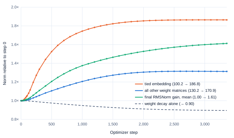
Part 5 kept weight decay on the tied embedding, the GPT-2 and nanoGPT convention, and promised to watch its norm, because OLMo 2 turned that decay off: it “overshoots the mark and results in very small embeddings,” which give large gradients in the early layers. Decay multiplies each decayed weight by 1 − 0.1 × lr every step; over this run’s schedule that compounds to 0.895, a 10.5% shrink if nothing pushed back.
Swipe to pan the diagram, or tap it to zoom.
The embedding didn’t shrink. Its norm grew 1.86 times, from 100.2 to 186.8 (a row’s mean length from 0.55 to 1.03), and stopped growing around step 2,500, when the learning rate was a quarter of its peak. The other matrices grew 1.31 times together; the MLP down-projections, initialized smaller, 3.8 times. The final RMSNorm’s gain, which isn’t decayed, rose to 1.61 and kept rising after the matrices stopped, so the output logits’ scale kept growing through the one weight decay doesn’t touch.
Tying explains part of it. The table is also the output layer, and the softmax gives every row a gradient on every step, even rows whose tokens never appear. That shows in the 55 token IDs that never occurred in the 1.76 billion training tokens: seven special tokens, among them <|user|> and <|assistant|>, plus { and 47 single bytes that are control characters or rare or invalid in UTF-8 text. Their rows grew from 0.55 to about 1.30, longer than average, because the output gradient pushes all of them the same way: away from the model’s hidden states, to keep their probabilities low. The seven special tokens ended with a pairwise cosine similarity of 0.90, against 0.18 for a typical pair of rows. As inputs they’re near-identical and untrained, which Part 10’s chat template will have to fix.
At this size and length, decaying the tied embedding did no visible harm, and the series keeps it.
In the real world
- PaLM’s 540B model saw “spikes in the loss roughly 20 times during training, despite the fact that gradient clipping was enabled,” which “were not observed when training the smaller models.” The fix was to restart “from a checkpoint roughly 100 steps before the spike started” and skip 200 to 500 batches. The same batches fed to an earlier checkpoint didn’t spike, so spikes came from “the combination of specific data batches with a particular model parameter state,” which is why the referee above uses more than one snapshot.
- OLMo 2 uses the same decay rule as
train.py, “every parameter is multiplied by 1 − (0.1 ⋅ lr) at every step,” and removed it from its embeddings, which, unlike ours, are a separate table from its output layer ("tie_word_embeddings": falsein the 7B model’s config). It also adds z-loss, a penalty that “keeps final output logits from growing too large,” the kind of growth the final norm gain above shows, mildly. - Pythia saved 154 checkpoints per model: at initialization, every 1,000 steps, and at log-spaced steps 1, 2, 4 and so on up to 512, for the same reason
--snapshot-atexists. - Olsson et al. (2022) found that induction heads, attention heads that copy what followed an earlier occurrence of the current token, form abruptly, “visible as a bump in the training loss,” around 2.5 to 5 billion tokens in their models. This run’s curve has no visible bump in 1.76 billion tokens; whether the heads formed anyway is a question for the snapshots.
- Hägele et al. (2024) found that a cosine schedule “underestimates the model’s performance” mid-run, because the rate hasn’t decayed yet. So a mid-run snapshot isn’t a finished model at that token count, and Part 8 gives each model size its own complete schedule.
Common misconceptions
- “A jump in the training loss is a loss spike.” The largest jump in this run, 0.20 at step 1,004, came with an ordinary gradient norm, and weights from before and after the step scored that batch 0.2 above its neighbours too. Check the gradient norm, the validation curve and, if snapshots exist, the batch itself.
- “Validation loss above training loss means overfitting.” In a single pass every training batch is unseen text, so there’s nothing to overfit. The 0.015 gap here came from which 655,360 tokens the check used: the whole shard is 0.017 easier.
- “Weight decay shrinks the weights.” On its own it would have shrunk them to 0.90 of their size over this run. With the gradients, the decayed embedding grew 1.86 times; decay only limited how far it grew.
- “Most of a long run’s value comes at the end.” The first 1.5% of the tokens bought half the loss drop and the first 30% bought 95%. The last 30% bought 0.07, and the samples still improved over it.
- “A loss of 3.37 can be compared with other models’ losses.” Only on the same tokenizer and text. Our 32,768-token vocabulary carries different amounts of text per token than GPT-2’s 50,257; Part 9 converts to bits per byte, which can be compared.
Key takeaways
- The 88M model trained on 1.76 billion tokens in 16 hours 49 minutes, in one try, at 29,399 tokens per second over its steps, within 0.03% of Part 6’s prediction and 72% MFU. The GPU used 0.83 kWh.
- Validation loss fell from 10.59 to 3.38, and 3.365 on the whole held-out shard: half the drop in the first 1.5% of tokens, then a long tail that flattened as the learning rate decayed.
- Training and validation losses stayed within a few hundredths of each other, because in a single pass over fresh data every training batch is held-out text.
- After warm-up only 12 steps were clipped, none after step 494, and the biggest jumps in the training loss were hard batches, as snapshots before and after confirmed.
- The model went from repeating one token, to “the the the”, to fluent English with invented facts. The weight-decayed tied embedding grew 1.86 times and settled, so the series keeps the decay.
What’s next
This run is one point: one model size, one budget. Part 8 trains five sizes on the laptop, each to its own compute-optimal budget, fits a power law through their final losses, and puts it next to Chinchilla’s, to test whether 20 tokens per parameter was the right call for an 88M model.
Further reading
- PaLM: Scaling Language Modeling with Pathways (Chowdhery et al., 2022): Section 5.1 on loss spikes at 540B parameters and the restart-and-skip fix.
- 2 OLMo 2 Furious (OLMo team, 2024): Section 3.4.2 on weight decay and embedding norms, and its other stability changes.
- Pythia: A Suite for Analyzing Large Language Models Across Training and Scaling (Biderman et al., 2023): 154 checkpoints per model, and studies that use them.
- In-context Learning and Induction Heads (Olsson et al., 2022): the phase change, visible as a bump in the loss, when induction heads form.
- Scaling Laws and Compute-Optimal Training Beyond Fixed Training Durations (Hägele et al., 2024): cosine versus constant learning rate with a cooldown, and what the decay does to the loss.
- Training Compute-Optimal Large Language Models (Hoffmann et al., 2022): the Chinchilla paper behind this run’s 20 tokens per parameter and its cosine length.
- Reproducing GPT-2 (124M) in llm.c in 90 minutes for $20 (Karpathy, 2024): the closest public run of this size.