
Inside the Model: Interpretability · Part 4 of 12
Attention Heads and Induction Heads, Measured in GPT-2
Find GPT-2 small's previous-token and induction heads, test how they compose, and measure what knocking them out does to in-context learning.
On this page
TL;DR
Each attention head decides where to look with one small matrix and what to copy with another. Some heads have jobs you can read off their attention patterns: one looks at the previous token, another at an earlier copy of the current token, and an induction head looks at the token that followed the earlier copy and predicts it again. This part finds those heads in GPT-2 small with repeated random tokens, shows that its induction heads read a previous-token head through their keys, and knocks them out. Removing five of 144 heads wrecks GPT-2’s copying of a repeated random sequence, while removing the top 12 takes only 18% to 27% of its in-context learning on real text. Pythia-160M and Qwen2.5-0.5B have induction heads too.
Why it matters
Show GPT-2 small 50 random tokens and it does worse than guessing: its loss, minus the natural log of the probability it gives the right token, averages 13.2 nats, while picking uniformly from its 50,257-token vocabulary would score 10.8. Show it the same 50 tokens again and the loss drops to 0.22 nats, which means it gives the right token about 80% probability on average. It knows nothing about these tokens; it is copying them from its own context.
That ability, using text earlier in the prompt to predict what comes next, is in-context learning, and it’s why a model can follow a format from three examples or pick up a made-up name. Olsson et al. (2022) argued that a particular kind of attention head, the induction head, is the mechanism behind most of it. In GPT-2 small, five heads score above 0.8 on the induction test. Knock out those five and the loss on the repeated half jumps from 0.22 to 5.5 nats. Knock out five other heads at random, 50 times over, and the median result is 0.25.
This part finds those heads, shows how they’re wired together, and measures how much of the model’s in-context learning on real text they carry.
The intuition
Picture reading a long contract and reaching “the Licensee shall”. A few pages back, the same three words were followed by “indemnify”. To guess the next word, you flip back, find the earlier “the Licensee shall”, and read the word after it.
That takes two clerks. The first walks through the document and puts a sticky note on every word saying which word came just before it. The second, standing at the current word, searches the notes for “the word before me was shall”, finds the note on “indemnify”, and reads that word out.
In a transformer, the first clerk is a previous-token head and the second is an induction head. Nobody programs them. Training builds them because copying repeated text lowers the loss.
The analogy breaks in two places. A real head doesn’t search for an exact match: it spreads its attention over every earlier token, and its “notes” are directions in a vector, not words. And the clerks don’t work alone: GPT-2 small has several heads doing each job, which matters once you start removing them.
Step 1: what one head computes
An attention head (Fundamentals Part 5) lets each token gather information from earlier tokens. For each destination token it produces an attention pattern, one weight per earlier source token, non-negative and summing to 1, and writes a weighted mix of what those tokens offer into the residual stream, the running vector per token that every layer reads from and adds to (Fundamentals Part 6).
Math Part 11 showed that a head’s four weight matrices collapse into two products. The QK circuit, W_Q W_Kᵀ, scores every pair of tokens and so decides where the head looks. The OV circuit, W_V W_O, decides what the head writes once it has looked. Anthropic’s A Mathematical Framework for Transformer Circuits (Elhage et al., 2021) made this split the basic unit of analysis: the QK circuit “determines which ‘source’ token the present ‘destination’ token attends back to,” while the OV circuit “describes what the resulting effect on the ‘out’ predictions for the next token is.”
Three head types matter here:
| Head type | Attends from the current token to | Score used here |
|---|---|---|
| Previous-token head | the token just before it | mean attention from token i to token i-1 |
| Duplicate-token head | an earlier copy of the same token | mean attention to the earlier copy |
| Induction head | the token after the earlier copy | mean attention to the earlier copy’s next token |
The scores follow Olsson et al.’s definitions. The previous-token score is measured on ordinary text. The other two need a sequence where every token appears exactly twice, so you know where the earlier copy is: a random sequence of tokens followed by the same sequence again.
The setup
The main model is GPT-2 small (openai-community/gpt2 on Hugging Face, 124 million parameters, MIT license): 12 layers of 12 heads, 144 in all, each working in 64 dimensions. It runs in fp32 through TransformerLens 3.9.0’s HookedTransformer.from_pretrained with its default weight processing on, which folds LayerNorm’s scale into the next weights and centers the weights that write to the residual stream. Outputs don’t change, but the QK and OV matrices below include LayerNorm’s scale. The hardware is an NVIDIA GeForce RTX 4060 Laptop GPU (8 GB) with PyTorch 2.11.
The repeated sequences are a beginning-of-sequence token followed by 50 random tokens and then the same 50 again, 101 tokens in all. Token IDs are drawn uniformly from 1,000 to 49,256, skipping the most common and the rarest entries in the vocabulary, as Olsson et al. also did. Heads are ranked on 200 sequences and measured on a separate 500 with a different seed, so the ranking can’t flatter itself. The previous-token score uses 200 windows of 255 tokens from WikiText-103 (CC BY-SA 4.0). Each 95% confidence interval below is ±1.96 standard errors over sequences.
Swipe to pan the diagram, or tap it to zoom.
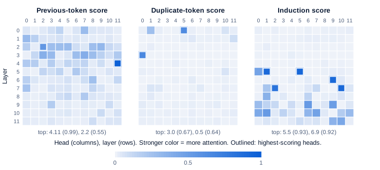
Each job lives in a few heads, and the layers fit a two-step mechanism: previous-token and duplicate-token heads sit in layers 0 to 4, induction heads only from layer 5 up.
| Head type | Top heads (score) | Heads that Wang et al. (2022) gave this role |
|---|---|---|
| Previous-token | 4.11 (0.99), 2.2 (0.55), 3.7 (0.39) | 2.2, 4.11 |
| Duplicate-token | 3.0 (0.67), 0.5 (0.64), 0.1 (0.27) | 0.1, 3.0, 0.10 |
| Induction | 5.5 (0.93), 6.9 (0.92), 7.10 (0.91), 5.1 (0.91), 7.2 (0.83) | 5.5, 6.9, 5.8, 5.9 |
Heads are written layer.head, counting from 0, and every score’s 95% CI is within ±0.006 except 0.1’s (±0.06). The right-hand column comes from Interpretability in the Wild (Wang et al., 2022), which found these head classes inside GPT-2 small’s circuit for indirect-object sentences by patching, a different method from this part’s attention scores. The two methods agree on the previous-token heads and on the two strongest induction heads. Below the top five, induction scores fall to 0.52 and spread thin: 12 heads score above 0.4, and the median head scores 0.005.
Step 2: the induction test, run
Random tokens make a clean test: with no grammar or topic to exploit, any drop in loss on the second copy has to come from looking back at the first. Here is the whole test, as run:
import torch
from transformer_lens import HookedTransformer

model = HookedTransformer.from_pretrained("gpt2", device="cuda")  # fp32, LayerNorm folded
torch.manual_seed(0)
r = torch.randint(1000, 49257, (100, 50))                  # 100 sequences of 50 random tokens
bos = torch.full((100, 1), model.tokenizer.bos_token_id)
tokens = torch.cat([bos, r, r], dim=1).cuda()               # [BOS] + r + r: 101 tokens

logits, cache = model.run_with_cache(tokens)
loss = -logits.log_softmax(-1)[:, :-1].gather(-1, tokens[:, 1:, None])[..., 0]
print(f"loss, first copy {loss[:, 1:50].mean():.2f}, second copy {loss[:, 51:].mean():.2f}")

d = torch.arange(51, 101)                                   # positions in the second copy
ind = torch.stack([cache["pattern", l][:, :, d, d - 49].mean((0, 2)) for l in range(12)])
top = ind.flatten().topk(5)
print([f"{i // 12}.{i % 12}: {v:.2f}" for v, i in zip(top.values.tolist(), top.indices.tolist())])
loss, first copy 13.16, second copy 0.23
['5.5: 0.93', '6.9: 0.92', '5.1: 0.91', '7.10: 0.91', '7.2: 0.83']The cache holds every head’s attention pattern, indexed [sequence, head, destination, source]. The token at position d in the second copy has its earlier copy at d - 50, so the token after that copy sits at d - 49: the induction score is the average weight on that one cell. This 100-sequence run has its own seed and finds the same five heads.
Token by token, the loss shows the copying switch on. On the 500-sequence set, the first token of the second copy still costs 11.8 nats, since nothing announces the repeat. The second costs 3.0, the third 1.4, the fourth 0.8, and the last ten average 0.08. One matching token is enough for the induction heads to lock on.
The OV side: do they copy?
The attention pattern says where an induction head looks. Whether it then predicts the attended token is the OV circuit’s job, and you can measure it directly. Direct logit attribution takes one head’s output vector at a position, scales it by the final LayerNorm as the model does, and dots it with the unembedding column of the correct next token. The result is how much that head alone raises the right answer’s logit, the raw score the model turns into a probability.
Averaged over the second copy of 200 sequences, the five induction heads raise the correct token’s logit by 0.30 (5.5), 1.09 (6.9), 1.18 (7.10), 0.68 (5.1) and 1.50 (7.2). On the first copy, where there’s nothing to copy, all five contribute 0.00, and on the second copy the median head contributes 0.001. Two weaker induction heads, 9.9 and 9.6, add 1.44 and 1.43. Head 5.5 has the sharpest attention but one of the smallest direct effects, a hint that much of its output feeds later heads instead of the logits. This says what each head writes, not whether the model needs it; that takes an ablation.
Step 3: how two heads cooperate
An induction head at the second “A” has to find the token whose previous token was “A”. Nothing in that token’s own embedding says so. The information has to be put there first, by a previous-token head that copies “A” into the residual stream at “B”. The induction head then reads it through its keys.
Elhage et al. call this K-composition: a later head’s key matrix reads a subspace that an earlier head wrote to. (Q-composition and V-composition are the same idea for queries and values.) Their paper says “the minimal way to create an induction head is to use K-composition with a previous token head to shift the key vector forward one token,” and found that the induction heads in their two-layer models were “totally reliant on a previous token head in the prior layer.”

You can look for this in the weights. The K-composition score from Elhage et al. measures how much of an earlier head’s OV output lands where a later head’s keys read: ‖W_QK^h2 W_OV^h1‖ / (‖W_QK^h2‖ ‖W_OV^h1‖), with Frobenius norms, the square root of the sum of squared entries. Two random matrices of the same shapes score 0.036 (standard deviation 0.0004 over 200 pairs). For each of the five induction heads, the top-scoring sender among all heads in earlier layers is 4.11, the 0.99 previous-token head, at 0.087 to 0.103, two to three times the median sender. Head 4.7 is a close second for all five, which the attention scores alone wouldn’t have flagged: its previous-token score is only 0.14.
A weight score is still only correlation. The causal test removes 4.11’s contribution from one place, the keys of the five induction heads, and leaves the rest intact: 4.11’s output minus its mean is subtracted from the input to those heads’ key projections, which TransformerLens exposes per head once use_split_qkv_input is on.
With 4.11 removed from their keys, the five heads’ average induction score falls from 0.90 to 0.41 and the second-copy loss rises from 0.22 to 2.91 nats (±0.07, 200 sequences). Removing previous-token head 2.2 as well brings the score to 0.26 and the loss to 4.78. As a control, the same surgery ran on each of the other 59 heads in layers 0 to 4, one at a time. The median one left the score at 0.90; the worst, head 3.7, brought it to 0.80. So about half of the induction heads’ attention to the right token depends on one sender, through one input.
Step 4: knocking the heads out
An ablation removes a component and measures what changes. Zero ablation sets a head’s output to zero, which can push the residual stream somewhere it never goes in normal use. Mean ablation, used here, replaces the head’s output (the z vector before the output projection) with its average over 200 reference sequences, so the head contributes its typical value but nothing about the current input. Zero-ablating the top five gives 4.95 nats where mean ablation gives 5.48, so the choice moves the result by about a tenth.
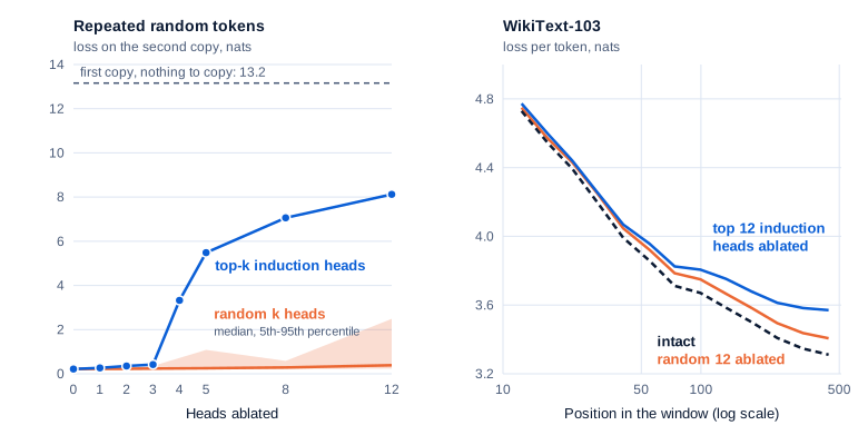
Each row ablates the top k induction heads, ranked on the selection set, and compares with 50 random sets of k heads drawn from the 132 heads outside the top 12. The metric is mean loss on tokens 2 to 50 of the second copy, over 500 sequences.
| Heads ablated | Top-k induction heads (95% CI) | Random k heads: median (5th to 95th percentile) |
|---|---|---|
| none | 0.22 (±0.01) | 0.22 |
| 1: 5.5 | 0.27 (±0.01) | 0.22 (0.21 to 0.31) |
| 2: + 6.9 | 0.35 (±0.01) | 0.22 (0.21 to 0.28) |
| 3: + 7.10 | 0.42 (±0.01) | 0.24 (0.20 to 0.36) |
| 4: + 5.1 | 3.32 (±0.04) | not run |
| 5: + 7.2 | 5.48 (±0.06) | 0.25 (0.20 to 1.08) |
| 8 | 7.06 (±0.06) | 0.29 (0.21 to 0.58) |
| 12 | 8.12 (±0.05) | 0.39 (0.23 to 2.49) |
Swipe to pan the diagram, or tap it to zoom.
The first three ablations cost little: 0.22 to 0.42 nats. Adding the fourth, 5.1, takes the loss to 3.32, and the fifth to 5.48. That’s redundancy: the heads back each other up, so the model fails only when nearly all of them are gone. Ablating any one of the five alone leaves the loss between 0.22 and 0.27, except 5.1, which raises it to 0.91. Keeping exactly one of the five and ablating the other four shows which heads can carry the load: 5.1 alone holds the loss at 0.74, while 5.5, 6.9, 7.2 or 7.10 alone leave it at 2.7, 2.5, 3.3 and 4.3.
A one-at-a-time sweep would conclude that only 5.1 matters. Wang et al. found similar backups among GPT-2’s name-mover heads. Random heads aren’t harmless either: one random set of five pushed the loss to 2.0 nats, which is why the comparison reports the median and the spread of 50 draws.
Step 5: in-context learning on real text
Real in-context learning means predicting ordinary text better as the context grows. Olsson et al. define the in-context learning score as “the loss of the 500th token in the context minus the average loss of the 50th token in the context, averaged over dataset examples.” A more negative score means later tokens are easier, so the model is using its context.
The test text is WikiText-103’s test and validation splits, cut into 976 windows of 512 tokens that each stay inside one article, from 120 articles. Windows from one article aren’t independent, so the 95% confidence intervals here come from a bootstrap that resamples whole articles (2,000 resamples).
GPT-2 small’s score is -0.78 nats (-1.04 to -0.51): the 50th token costs 3.98 nats on average, the 500th 3.20. Olsson et al. reported about 0.4 nats for their own models and data, so the two aren’t directly comparable.
| Ablation (mean, 976 windows) | In-context learning score | Change vs. intact (95% CI) | Loss over all tokens |
|---|---|---|---|
| none | -0.78 | 3.56 | |
| top 5 induction heads | -0.69 | +0.09 (0.05 to 0.14) | 3.65 |
| 5 random heads, 5 draws | -0.75 to -0.80 | -0.02 to +0.03 | 3.58 to 3.62 |
| top 12 induction heads | -0.64 | +0.14 (0.08 to 0.21) | 3.75 |
| 12 random heads, 5 draws | -0.71 to -0.76 | +0.02 to +0.07 | 3.62 to 3.67 |
Knocking out the top 12 induction heads removes about 18% of GPT-2’s in-context learning on Wikipedia text, against 2% to 9% for random sets of 12: specific, and far from “most”. On repeated random tokens, the same 12 heads cut the geometric-mean probability of the right token on the second copy from 80% to 0.03%.
A single token’s loss is noisy, so a smoothed version uses mean loss over tokens 491 to 510 minus tokens 41 to 60, per window. GPT-2’s gap is -0.64 nats (-0.72 to -0.56). Ablating the top 12 induction heads shrinks it by 0.17 (0.15 to 0.20), about 27%; two random sets of 12 shrink it by 0.02 and 0.08.
The damage is uneven. In this WikiText sample, 17% of tokens are ones an induction head could predict outright: the current token appeared earlier in the window, followed then by the same token that comes next now. GPT-2 predicts those at 1.22 nats against 4.03 for everything else. Ablating the top 12 induction heads raises the loss on those tokens by 0.67 nats (0.63 to 0.72) and on all other tokens by only 0.09 (0.08 to 0.09). Two random sets of 12 raise the two groups by 0.17 and 0.16, and by 0.14 and 0.08, a small cost spread over every kind of token.
On random tokens, exact copying is the only signal. On real text, the context helps in other ways too: the topic narrows the vocabulary, and a name’s first mention makes later ones likely. And an ablation measures only what the model can’t route around.
Step 6: other models
The same search ran on two more models with the same seeds and lengths: Pythia-160M (EleutherAI/pythia-160m, Apache-2.0; 12 layers of 12 heads, fp32, same weight processing) and Qwen2.5-0.5B (Qwen/Qwen2.5-0.5B, Apache-2.0; 24 layers of 14 query heads sharing 2 key-value heads, bf16, loaded with from_pretrained_no_processing because folding its weights needs more host memory than this machine allows). Qwen has no beginning-of-sequence token, so its end-of-text token starts each sequence.
Pythia needed one change. Uniformly drawn IDs include tokens it barely saw in training, which it scored at up to 826 nats, swamping every average, so its random tokens come from the 9,963 tokens that appear at least 5 times in the WikiText sample. Its second-copy loss still varies far more between sequences than the other models’.
| Measurement (500 repeated sequences) | GPT-2 small | Pythia-160M | Qwen2.5-0.5B |
|---|---|---|---|
| Heads | 144 | 144 | 336 |
| Loss on first copy, nats | 13.16 | 13.80 | 14.59 |
| Loss on second copy, nats | 0.22 | 2.17 (±0.35) | 0.58 (±0.02) |
| Heads with induction score above 0.4 | 12 | 14 | 14 |
| Strongest induction heads | 5.5, 6.9, 7.10 (0.91 to 0.93) | 4.6, 8.2, 4.10 (0.90 to 0.98) | 16.3, 11.12, 16.2 (0.95 to 0.98) |
| Strongest previous-token head | 4.11 (0.99) | 3.2 (0.87) | 8.7 (0.88) |
| Second-copy loss, top 5 induction heads ablated | 5.48 | 9.43 | 0.94 |
| Same, 5 random heads (median) | 0.25 | 2.30 | 0.60 |
| Second-copy loss, top 12 ablated | 8.12 | 11.59 | 8.74 |
| Same, 12 random heads (median) | 0.39 | 2.84 | 0.68 |
The random rows use 50 draws for GPT-2 and 10 for the others. In all three, induction heads sit just above a strong previous-token head: layer 4 above 3.2 in Pythia, layer 9 above 8.7 in Qwen. Qwen spreads the job wider: without its top five the loss only rises from 0.58 to 0.94, and it takes the top eight (5.32 nats) to break it.
On WikiText, ablating the top 12 shrinks the exact in-context learning score by 0.21 nats (0.14 to 0.29) in Pythia, against 0.01 and 0.12 for two random sets, and by 0.09 (0.02 to 0.15) in Qwen, against -0.05 for one random set. Qwen’s single-token score is too noisy on 400 windows to read (-0.02, CI -0.38 to 0.38); its smoothed gap is -0.51 nats intact and -0.40 with the top 12 ablated.
In the real world
Olsson et al. tracked 34 transformers, up to 13 billion parameters, through training, ran more than 50,000 head ablations, and found that in-context learning “develops abruptly in a narrow window early in training (roughly 2.5 to 5 billion tokens),” rising from under 0.15 nats to roughly 0.4, at the same time as induction heads form. Their ablations were run on small models; for large models with MLPs, the authors write, “we must therefore rely on mainly correlational evidence, which could be confounded.” Part 10 of this series looks for that formation in the checkpoints of the From Scratch model, whose pretraining run showed no visible bump in 1.76 billion tokens.
In GPT-2 small itself, Wang et al. found induction heads 5.5 and 6.9 and previous-token heads 2.2 and 4.11 inside the indirect-object circuit, where the induction heads’ outputs serve as a position signal for later heads.
In bigger models, Bansal et al. (2022) found that “~70% of attention heads and ~20% of feed forward networks can be removed with minimal decline in task performance” in OPT-66B, and that “a small set of attention heads in OPT-66B score highly on their ability to perform primitive induction operations.” Crosbie and Shutova (2024) ablated induction heads in Llama-3-8B and InternLM2-20B and report that “minimal ablation of induction heads leads to ICL performance decreases of up to ~32%” on abstract pattern-recognition tasks, bringing performance close to random. These are published results, not reproduced here.
Common misconceptions
- “An attention pattern tells you what a head does.” It tells you where the head looks. Head 4.7 puts only 14% of its attention on the previous token, yet it’s the second-strongest sender into every induction head’s keys by weight. What a head contributes needs an intervention, like the key-path ablation above.
- “If ablating a head barely hurts, the head doesn’t matter.” Ablating GPT-2’s best induction head raised the second-copy loss from 0.22 to only 0.27, because four other heads cover for it. Removing all five raised it to 5.48. Single-head ablations miss redundant mechanisms.
- “Induction heads are the model’s in-context learning.” On repeated random tokens, nearly all of it. On Wikipedia text, ablating the top 12 removed about 18% of GPT-2’s in-context learning score. Olsson et al. argued for “most” in their own models, and called their large-model evidence mainly correlational.
- “Random-token tests show how a model behaves on real text.” They isolate one mechanism by removing everything else, which makes them clean and also makes them overstate how much it matters in normal use.
- “Each head has one job.” Heads 5.5 and 6.9 copy in random sequences and supply a position signal in GPT-2’s indirect-object circuit. A role describes what a head does on some inputs.
Key takeaways
- An attention head is two circuits: QK decides where it looks and OV decides what it writes. Attention scores on designed inputs reveal previous-token, duplicate-token and induction heads directly.
- GPT-2 small has five strong induction heads, 5.5, 6.9, 7.10, 5.1 and 7.2, scoring 0.83 to 0.93. They cut the loss on a repeated random sequence from 13.2 nats to 0.22.
- Induction heads read a previous-token head through their keys. In GPT-2 that’s head 4.11: removing it from just their keys halves their induction score, from 0.90 to 0.41, while no other early head moves it below 0.80.
- The heads back each other up: ablating three raises the loss to 0.42, ablating five to 5.5. On real text, ablating the top 12 removes 18% to 27% of the in-context learning score, and the damage concentrates on the 17% of tokens that repeat an earlier pair.
- The same test finds induction heads just above a strong previous-token head in Pythia-160M and Qwen2.5-0.5B. Qwen has more backups: it needs eight ablated before copying fails.
What’s next
Ablation asks what happens when a component disappears. Part 5 asks a sharper question with activation patching: take one activation from a run where the model gets the answer right, paste it into a run where it doesn’t, and see whether the right answer comes back. That’s how researchers traced where GPT-2 XL recalls facts, and how the indirect-object circuit was found.
Further reading
- In-context Learning and Induction Heads (Olsson et al., 2022): the six arguments that induction heads drive in-context learning, the phase change, and the score definitions used here. Also on arXiv.
- A Mathematical Framework for Transformer Circuits (Elhage et al., 2021): QK and OV circuits, Q-, K- and V-composition, and induction heads in two-layer attention-only models.
- Interpretability in the Wild: a Circuit for Indirect Object Identification in GPT-2 small (Wang et al., 2022): GPT-2 small’s previous-token, duplicate-token and induction heads inside a larger circuit, found by patching.
- Rethinking the Role of Scale for In-Context Learning (Bansal et al., 2022): head pruning and induction heads in OPT-66B.
- Induction Heads as an Essential Mechanism for Pattern Matching in In-context Learning (Crosbie and Shutova, 2024): induction-head ablations in Llama-3-8B and InternLM2-20B.
- TransformerLens: the library used for every hook, cache and ablation in this part.
- Pythia: A Suite for Analyzing Large Language Models Across Training and Scaling (Biderman et al., 2023): the open model family used for the repeat test, with public training checkpoints.
- Qwen2.5 Technical Report (Qwen Team, 2024): the modern model used for the repeat test.