
Inside the Model: Interpretability · Part 7 of 12
Sparse Autoencoders: Pulling Features Out of a Model
Train a sparse autoencoder on GPT-2 small on a laptop, compare it with public ones, then explore and score Gemma Scope features on Gemma 2 2B.
On this page
TL;DR
A sparse autoencoder (SAE) rewrites each of a model’s activation vectors as a short sum of directions picked from a large learned dictionary, so that each direction, with luck, means one thing. This part trains three SAEs on layer 8 of GPT-2 small in 43 minutes on a laptop GPU and measures how many latents fire per token, how much of the activation they rebuild, and how much worse the model predicts text when the rebuild replaces the real activation. The best one, a TopK SAE with 24,576 latents, explains 84.9% of the variance and costs 0.11 nats of next-token loss, slightly better than two public SAEs on the same text. Then it explores a Gemma Scope SAE on Gemma 2 2B: 50 random latents scored by hand (66% clearly interpretable) and one clamped to steer the model, a preview of Part 9.
Why it matters
Ask what one GPT-2 neuron does and you usually get a shrug: it fires on several unrelated things. Fundamentals Part 16 and Part 6 of this series explain why. A model represents more features than it has dimensions, packing them in as nearly perpendicular directions, so no single neuron lines up with any one of them.
A sparse autoencoder is built to undo that packing. Of 50 latents drawn at random from a Gemma Scope SAE on Gemma 2 2B, 33 had top examples that shared one nameable idea: the word “surface”, birth dates, “All rights reserved” lines, ancient Egypt. Clamping the Egypt latent turned “The teacher asked the class to” into “…write a poem about the Nile River.”
The same experiments show the cost. Our best rewrite of GPT-2’s layer 8 leaves 15% of the variance unexplained, and splicing it in raises the model’s perplexity by 12%.
The intuition
Think of every activation vector as a smoothie, and the SAE as someone trying to write down the recipe. They have a pantry of 24,576 jars, and they must describe each smoothie using only a few jars, with an amount for each: two scoops of banana, a little spinach, nothing else. Training means stocking the pantry so that every smoothie in a huge pile can be described that way and tastes right when remade.
Sparsity is the “only a few jars” rule. Without it, a recipe could use a pinch of every jar and no jar would mean anything.
The analogy breaks in three places. Nobody hands the SAE a list of real ingredients; it invents the jars, and a bigger pantry splits one jar into several. A remade smoothie never tastes quite the same, and the leftover difference is real flavor the recipe missed. And a jar’s label is a guess made by someone reading where it gets used, not a fact about the model.
Step 1: what an SAE computes
An SAE is a two-layer network trained on activations saved from a frozen model, here the residual stream (the running vector per token that every layer reads from and adds to, from Part 2). For one activation x with d numbers:
f  = σ(W_enc x + b_enc)      encoder: one number per latent, most of them 0
x̂  = W_dec f + b_dec         decoder: rebuild x from the active latents
W_enc has one row per latent and W_dec one column per latent, and a dictionary is usually much wider than d: 24,576 latents for GPT-2’s 768 dimensions here. Each column of W_dec is that latent’s direction in the model’s space, and f says how much of each direction to add. People call the entries of f “latents” or “features”; this article says latent for the SAE’s unit and feature for the property it might track.
The activation function σ decides how sparsity is enforced. Three choices are common:
- ReLU (rectified linear unit) sets negatives to 0 and keeps everything else. On its own it leaves many small values on, so training adds an L1 penalty, a cost proportional to the total size of the activations. Fundamentals Part 16 worked through how that penalty shrinks every active latent and switches off weak ones.
- TopK, from Gao et al. (2024) at OpenAI, keeps exactly the
klargest values per token and zeroes the rest. The authors note it “removes the need for the L1 penalty”, since sparsity is fixed by construction. - JumpReLU, from Rajamanoharan et al. (2024) at Google DeepMind, keeps a value only if it clears a learned threshold per latent. It is trained with a penalty on L0, the number of active latents, directly, “avoiding problems like shrinkage.”
Here they are on six made-up encoder outputs:
import torch

pre = torch.tensor([3.1, 0.2, -1.0, 1.8, 0.4, 0.0])   # encoder outputs for 6 latents

relu = pre.clamp(min=0)                                # ReLU: keep every positive value
v, i = pre.topk(2)                                     # TopK with k = 2: keep the 2 largest
topk = torch.zeros_like(pre).scatter(0, i, v.clamp(min=0))
jump = torch.where(pre > 1.0, pre, 0.0)                 # JumpReLU with threshold 1.0

for name, f in [("ReLU", relu), ("TopK", topk), ("JumpReLU", jump)]:
    print(f"{name:8s} {[round(x, 1) for x in f.tolist()]}  L0 = {int((f > 0).sum())}")
ReLU [3.1, 0.2, 0.0, 1.8, 0.4, 0.0] L0 = 4
TopK [3.1, 0.0, 0.0, 1.8, 0.0, 0.0] L0 = 2
JumpReLU [3.1, 0.0, 0.0, 1.8, 0.0, 0.0] L0 = 2L0 is the standard sparsity measure: how many latents are on for a token, averaged over tokens. ReLU lets the two weak values through, which is why it needs a penalty to push them down. TopK and JumpReLU cut them without touching the strong ones.
Dead latents and feature splitting
Two problems show up in every SAE paper. A dead latent is one that stops firing early in training and never recovers; its parameters are wasted. Towards Monosemanticity (Bricken et al., 2023) reset dead latents by hand during training, and still found 168 of its 4,096 features “active on none of the 100 million dataset examples”. Gao et al. initialize the encoder as the transpose of the decoder and add a second loss term, AuxK, that makes dead latents explain some of the leftover error, and report that “even in our largest (16 million latent) autoencoder only 7% of latents are dead.”
Feature splitting is what happens as the dictionary grows. In Bricken et al.’s one-layer model, “the number of features specific to base64 contexts goes from 1 to 3 to many more” as the dictionary went from 512 to 4,096 to 16,384 latents. No size is the right one; each gives a different level of detail.
How you judge an SAE
Papers judge an SAE by three numbers, and this article reports all three:
- L0, as above.
- Fraction of variance explained (FVE): one minus the rebuild’s total squared error divided by the activations’ total squared deviation from their mean. 100% is a perfect rebuild.
- Downstream loss: put
x̂back into the model in place ofx, run the rest of the forward pass, and measure the next-token cross-entropy (from Math Part 6). Gao et al. report the difference from the unaltered model, “delta cross-entropy”, and Gemma Scope calls it “delta LM loss”.

The spliced loss matters most: a rebuild can be close in squared error and still drop the part of the vector later layers rely on.
Step 2: training our own SAE on GPT-2 small
GPT-2 small (openai-community/gpt2, 124 million parameters, MIT license) runs in fp32 through TransformerLens 3.9.0’s HookedTransformer.from_pretrained, with its default weight processing on (LayerNorm folded, writing weights centered, as in Parts 1 and 4). The SAEs read blocks.8.hook_resid_pre, the residual stream entering block 8 of 12, the layer Gao et al. and both public SAEs below also used.
The training text is FineWeb-Edu (ODC-By 1.0), the sample-10BT subset the From Scratch series downloaded: 83,000 documents cut into windows of 127 tokens with GPT-2’s <|endoftext|> token in front. The start token’s vector is identical in every window and far longer than any other (Part 2 measured 40 times by block 3), so every SAE here skips it. Activations were computed on the fly and shuffled within chunks of 260,000 tokens.
We trained three SAEs side by side on the same 29.9 million activations, 7,300 steps of 4,096 tokens, with Adam:
| SAE | Latents | Sparsity | Learning rate |
|---|---|---|---|
| TopK | 24,576 | exactly 32 active per token | 0.0002 |
| TopK | 3,072 | exactly 32 active per token | 0.0004 |
| ReLU with L1 | 24,576 | L1 coefficient 15 | 0.0002 |
The ReLU recipe follows Anthropic’s April 2024 update: activations scaled by one constant, an L1 penalty weighted by each latent’s decoder norm, the coefficient ramped up over the first 5% of steps, no resampling of dead latents. In a pilot with coefficients 5, 10 and 20, L0 after 700 steps was 264, 152 and 64, still falling slowly, so we picked 15. The TopK SAEs use Gao et al.’s AuxK loss with their settings, 512 auxiliary latents and a weight of 1/32, counting a latent as dead after 4 million tokens without firing.
Training ran on an NVIDIA GeForce RTX 4060 Laptop GPU (8 GB) with PyTorch 2.11, TopK in bf16 autocast and ReLU in TF32, at a peak of 7.1 GB of GPU memory. It took 2,603 seconds, about 43 minutes, in two pieces: the first hit its 38-minute time limit at step 6,517 and resumed from a checkpoint. The code, lab/sae.py, is about 300 lines.
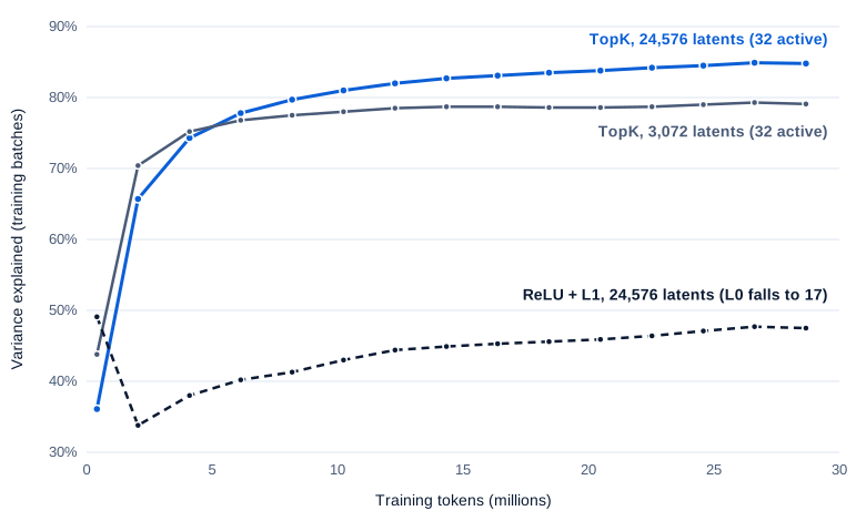
Swipe to pan the diagram, or tap it to zoom.
The small dictionary learns fastest, then runs out of room. The large TopK SAE overtakes it after 5 million tokens and was still improving when we stopped.
Ours against two public SAEs
We compared against two public SAEs at the same hook, loaded with SAELens 6.54.12 (MIT license):
gpt2-small-res-jb, Joseph Bloom’s 2024 ReLU SAEs, 24,576 latents, trained with “an L1 coefficient of 8e-5, a learning rate of 4e-4 for 300 Million tokens from OpenWebText” (Bloom, 2024).gpt2-small-resid-post-v5-32k, OpenAI’s TopK SAEs from Gao et al. (released code and weights), 32,768 latents withk = 32, atblocks.7.hook_resid_post, which is the same tensor.
The test set is Part 2’s 586 held-out FineWeb-Edu documents, 4,231 windows and 537,337 scored tokens, none of them seen in training. Intervals are 95% bootstrap intervals over documents (2,000 resamples). Unaltered, GPT-2 small scores 3.697 nats per token (3.645 to 3.752).
| SAE (GPT-2 small, layer 8) | Latents | L0 | Variance explained | Spliced loss, nats | Delta loss, nats |
|---|---|---|---|---|---|
| Ours, TopK | 24,576 | 32 | 84.9% (84.7 to 85.1) | 3.811 | 0.114 (0.110 to 0.117) |
| Ours, TopK | 3,072 | 32 | 79.2% (79.1 to 79.4) | 3.896 | 0.199 (0.194 to 0.205) |
| Ours, ReLU with L1 | 24,576 | 17.3 | 47.8% (47.5 to 48.1) | 4.741 | 1.044 (1.027 to 1.061) |
| Bloom, ReLU | 24,576 | 70.7 | 84.0% (83.9 to 84.2) | 3.896 | 0.199 (0.193 to 0.206) |
| OpenAI, TopK | 32,768 | 32 | 84.9% (84.8 to 85.0) | 3.831 | 0.134 (0.130 to 0.138) |
The gap between “reconstructs well” and “the model doesn’t notice” is large. Our best SAE leaves 15% of the variance unexplained, and the model’s loss goes up by 0.114 nats, which multiplies perplexity by about 1.12. A common way to make that look small is to compare it with replacing the activation by zeros, which costs 7.65 nats: on that scale our SAE “recovers” 98.5% of the loss. Gao et al. warn that with this kind of score “even very poorly explaining the behavior can result in high scores”, which is why the table reports the delta instead.
TopK beat L1 at this training length by a wide margin. The ReLU SAE spent its 30 million tokens pushing L0 down, from 2,231 at the start to 17, and its rebuild never caught up; the pilot runs with weaker penalties were still far denser. Anthropic’s update gives 200,000 steps as a default, 27 times our run, so this says more about short runs than about L1 at scale. TopK sidesteps the problem by fixing L0 from step one.
The public SAEs come close, and home advantage explains part of the gap. Ours were trained on FineWeb-Edu, the same kind of text as the test set, while both public SAEs were trained on OpenWebText, and OpenAI’s used windows of 64 tokens against our 128. Bloom’s post reports 92.6% variance explained at layer 8 on its own data; on ours it explains 84.0%. An SAE’s scores belong to a distribution, not just to the SAE.
How often each latent fires
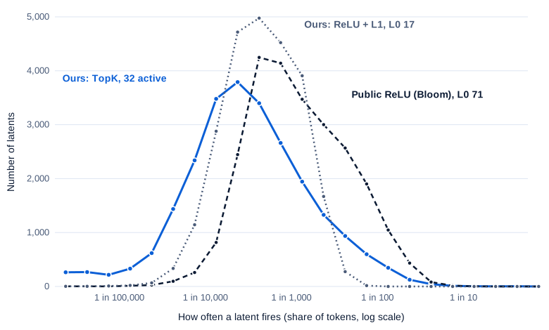
Swipe to pan the diagram, or tap it to zoom.
TopK spreads its latents widest, from very rare to frequent, because it never charges a latent for being used. The L1 penalty keeps every latent in a narrow middle band.
Silence on half a million test tokens doesn’t make a latent dead: during training only 30 of our 24,576 TopK latents (0.12%) went 4 million tokens without firing. Most of the 433 silent ones are just very rare. At the other end, 11 of the TopK latents fire on more than 10% of tokens, close to always on.
Feature splitting, measured
Our 3,072-latent and 24,576-latent SAEs were trained on the same activations, so their decoder directions can be compared with cosine similarity (1 means the same direction). For the median small-SAE latent, the closest large-SAE latent has a cosine of 0.72. Only 12% of small latents have a near copy above 0.9, and 55% have two or more large latents above 0.5.
One example: small latent 533 fires on medical imaging tokens, ” ultr” in “ultrasonography”, ” imaging” in “magnetic resonance imaging”, and “ray” in “X-ray”. In the large SAE its nearest neighbors split the theme three ways. Latent 3783 (cosine 0.69) fires on ” include” in “Tests may include:”. Latent 15887 (0.61) fires on ” exam” in “a physical exam”. Latent 10178 (0.61) fires on pieces of “electrocardiogram” and “electroencephalogram”. Which of these counts as “the” feature depends on the dictionary size you chose.
Step 3: Gemma Scope on Gemma 2 2B
Good SAEs for a modern model take far more compute than a laptop has. Gemma Scope (Lieberum et al., 2024) released “more than 400 sparse autoencoders” for Gemma 2, all JumpReLU, under CC-BY-4.0; the 16,384-latent ones were “trained for 4B tokens”, 130 times our GPT-2 run. We downloaded one: google/gemma-scope-2b-pt-res, layer_12/width_16k/average_l0_82 (302 MB), the residual stream after layer 12 of 26. Its model card calls the SAE with average L0 closest to 100 the canonical one, and this is it.
The model is Gemma 2 2B (google/gemma-2-2b, released under the Gemma Terms of Use), loaded in bf16 straight to the GPU with plain Hugging Face transformers 5.21.1, no weight processing, which used 5.5 GB of GPU memory. Following Gemma Scope, which collected activations only “from tokens which are neither BOS, EOS, nor padding”, we skip the start token (BOS).
On 500 held-out documents of 255 tokens each, the SAE runs at L0 85.0 and explains 78.0% of the variance. Splicing it into layer 12 raises Gemma’s loss from 2.414 to 2.515 nats, a delta of 0.100 (0.096 to 0.104), slightly less than our best GPT-2 SAE.
Then we ran 2.04 million tokens from 8,000 other FineWeb-Edu documents through the model and kept every latent’s 20 strongest activations. Only 23 of the 16,384 latents never fired; 1,224 fired fewer than 50 times.
What the latents look like
Six latents from the random sample below, each with its strongest token in brackets and a few words of FineWeb-Edu context:
| Latent | Strongest example | Fires on |
|---|---|---|
| 3476 | small changes in [surface] temperature | 0.11% of tokens |
| 8834 | was born on 23rd [July] 190... | 0.32% |
| 9234 | University of Cambridge. [All] rights reserved. | 0.007% |
| 10296 | the offspring is always sterile (like the [mule]) | 1.1% |
| 6252 | go with the flow and [let] the universe carry you | 0.063% |
| 7498 | used by the ancient [Egy]ptians in building | 0.86% |
Some are words, some are formats, and some cut across words: latent 10296’s top examples include “Mixed-race”, “mestizo”, “hybrid”, “griffin” and “purple” made “by mixing two primary colors”.
Scoring 50 random latents
Hand-picked latents flatter SAEs, so we also drew 50 latents uniformly at random (seed 7) and scored each from its 10 strongest activations plus 5 drawn at random from all its nonzero activations. The rubric:
- 2, clear: the top 10 share one specific concept you can name in a few words.
- 1, partial: a broad, structural or partly mixed theme that at least 6 of the 10 fit.
- 0, none: no common theme.
Separately, we counted how many of the 5 random activations clearly fit the same concept. The rater was the writer of this article, an AI model, unblinded and alone, so treat the shares as one careful reading, not a benchmark.
| 50 random Gemma Scope latents | Share (95% Wilson interval) |
|---|---|
| Clear (2) | 66% (52 to 78%) |
| Partial (1) | 24% (14 to 37%) |
| None (0) | 10% (4 to 21%) |
| At least 3 of 5 random activations fit | 24% (14 to 37%) |
The none group is mostly latents that barely fire: 3 of the 5 fired fewer than 25 times in 2 million tokens. Among the 44 latents that fired at least 50 times, 32 (73%) were clear. The partial ones are often structural, like “a comma joining two clauses” or “the token right after a place name”.
The last row matters most. A latent’s label describes its strongest activations, and at ordinary strengths, often a tenth to a fifth of the maximum, only a quarter of latents still clearly track the same thing. Bricken et al. scored each feature separately across intervals of activation strength, and on their 14-point rubric “the median neuron scored 0” while “the median feature interval scored a 12”, in their one-layer model.
A causal check: clamping the Egypt latent
If latent 7498 means “Egypt”, forcing it on should make Gemma talk about Egypt. We clamped it: at layer 12, at every position after the start token, we set its activation to a value c by adding (c - f) × direction to the residual stream, which keeps the SAE’s error term untouched. Then we generated 30 tokens greedily from 20 neutral prompts and counted completions mentioning Egypt, the Nile, a pharaoh, Cairo or a pyramid. The latent’s strongest natural activation was 25.4.
Clamp value c | Completions mentioning Egypt (of 20) |
|---|---|
| none | 0 |
| 25 (1 times the max) | 0 |
| 50 | 1 |
| 75 | 3 |
| 100 (4 times) | 4 |
| 125 | 3 |
| 150 | 0, text starts to degrade |
| 250 (10 times) | 0, text is broken (“have have have…”) |
At c = 100, “Scientists recently discovered that” continued with “the ancient Egyptian pyramids were built to be used as tombs for the pharaohs.” At c = 50, “On our trip we decided to” became “visit the city of Cairo.” The keyword count is conservative: at c = 125 one completion was about “the life of Cleopatra” and wasn’t counted. Still, the clamp works weakly: at best 4 of 20 completions (20%, Wilson interval 8 to 42%), in a narrow window between no effect and breaking the model. Anthropic clamped its Golden Gate Bridge feature to 10 times its maximum in Claude 3 Sonnet with a 34-million-latent SAE (Templeton et al., 2024); in Gemma 2 2B, 10 times broke the output. Part 9 covers steering properly, with side effects measured.
In the real world
- Anthropic’s Scaling Monosemanticity trained SAEs with “1,048,576 (~1M), 4,194,304 (~4M), and 33,554,432 (~34M) features” on Claude 3 Sonnet’s middle layer, with “an L1 coefficient of 5”. Dead features rose from “roughly 2% for the 1M SAE” to “65% for the 34M SAE”, and “a ‘San Francisco’ feature in the 1M SAE splits into two features in the 4M SAE and eleven fine-grained features in the 34M SAE.” Not reproduced here.
- OpenAI’s Gao et al. trained “a 16 million latent autoencoder on GPT-4 activations for 40 billion tokens” and found that, spliced in, it gives “a language modeling loss corresponding to 10% of the pretraining compute of GPT-4.” Not reproduced here.
- Gemma Scope used “over 20% of the training compute of GPT-3”. On Gemma 2 9B, the JumpReLU paper reports “reconstructions that are at least as good as, and often slightly better than, TopK SAEs.”
- Engels et al. (2024) found that “about half of the error vector itself and > 90% of its norm” can be predicted linearly from the input activation, so much of this “dark matter” is structure the SAE missed.
- SAEs can learn latents that skip cases they seem to cover. Chanin et al. (2024) named this feature absorption: a latent “fails to activate on seemingly arbitrary tokens” because “more specific latents” absorb the feature, which happens “whenever the underlying features form a hierarchy.”
- For practical detection, a plain probe often wins. As Part 3 noted, Google DeepMind’s team found that SAE-based probes underperformed linear probes at detecting harmful intent on Gemma 2 9B, especially out of distribution, and said it was “deprioritising fundamental SAE research for the moment”.
Common misconceptions
- “An SAE’s latents are the model’s true features.” They depend on the dictionary. Our 3,072-latent SAE’s medical-imaging latent became at least three latents at 24,576, and only 12% of small latents had a near copy in the large one.
- “High variance explained means the SAE captures what the model computes.” Our best GPT-2 SAE explained 84.9% and still raised the loss by 0.114 nats, and Bloom’s SAE scored 92.6% on its own data but 84.0% on ours. Splicing the SAE in is the test that counts.
- “98% of the loss recovered sounds nearly perfect.” That figure compares the SAE with zeroing the activation, a baseline 7.65 nats worse than the real model. The same SAE multiplies perplexity by 1.12.
- “If a latent’s top examples all mean one thing, the latent means that thing.” At typical strengths only about a quarter of our sampled latents still clearly fit their label. A label describes the top of the range.
- “Finding a latent means you can steer with it.” Clamping the Egypt latent moved at most 4 of 20 completions, at a strength close to the one that breaks the text.
Key takeaways
- A sparse autoencoder rebuilds each activation from a few directions out of a large dictionary. ReLU with an L1 penalty, TopK and JumpReLU are three ways to keep it sparse, and they trade differently between shrinkage, tuning and dead latents.
- Judge an SAE by three numbers together: how many latents fire per token, how much variance the rebuild explains, and how much the model’s loss rises when the rebuild replaces the real activation.
- On a laptop, a TopK SAE trained on 30 million tokens of GPT-2’s layer 8 in 43 minutes reached 84.9% variance explained at 32 active latents and a loss increase of 0.11 nats, a little better than two public SAEs on the same text. An L1 SAE trained the same way fell far short.
- Gemma Scope’s layer-12 SAE on Gemma 2 2B gives readable latents: 66% of a random 50 were clearly interpretable at their strongest activations, though only a quarter stayed on-theme at typical strengths.
- Every SAE leaves an error that matters to the model, and its latents change with the dictionary size, so check any reading with an intervention.
What’s next
An SAE lists the features at one layer but not how they connect. Part 8 uses transcoders, SAE-like stand-ins for a model’s MLPs, to draw attribution graphs: which features, at which layers, pushed the model toward its answer on one prompt. It tests whether the open-source circuit-tracer tools fit an 8 GB laptop GPU and checks a traced path by intervening on it.
Further reading
- Towards Monosemanticity: Decomposing Language Models With Dictionary Learning (Bricken et al., 2023): the first convincing SAE results, on a one-layer model, with feature splitting, dead features and a scoring rubric.
- Scaling Monosemanticity: Extracting Interpretable Features from Claude 3 Sonnet (Templeton et al., 2024): SAEs with up to 34 million latents on a production model, and the Golden Gate Bridge clamp.
- Circuits Updates, April 2024: how Anthropic trains SAEs: the decoder-norm-weighted L1 recipe used for our ReLU SAE.
- Scaling and evaluating sparse autoencoders (Gao et al., 2024): TopK SAEs, the AuxK loss, delta cross-entropy, and the 16 million-latent SAE on GPT-4.
- Jumping Ahead: Improving Reconstruction Fidelity with JumpReLU Sparse Autoencoders (Rajamanoharan et al., 2024): thresholded activations trained with an L0 penalty.
- Gemma Scope: Open Sparse Autoencoders Everywhere All At Once on Gemma 2 (Lieberum et al., 2024): the open SAEs explored in Step 3.
- Decomposing The Dark Matter of Sparse Autoencoders (Engels et al., 2024): what the reconstruction error contains.
- A is for Absorption: Studying Feature Splitting and Absorption in Sparse Autoencoders (Chanin et al., 2024): latents that silently miss part of their feature.
- Negative Results for SAEs On Downstream Tasks and Deprioritising SAE Research (Google DeepMind, 2025): where SAE probes lost to linear probes.
- Open Source Sparse Autoencoders for all Residual Stream Layers of GPT2-Small (Bloom, 2024): the public ReLU SAEs we compared against.
- openai/sparse_autoencoder (GitHub): OpenAI’s TopK SAEs for GPT-2 small.
- SAELens (GitHub): the MIT-licensed library used to load the public SAEs.
- Inside the Black Box: Features, Superposition and Circuits (Fundamentals Part 16): the series overview, with the L1 penalty worked by hand.