
Inside the Model: Interpretability · Part 6 of 12
Superposition: How Models Store More Features Than Neurons
Reproduce Toy Models of Superposition on a laptop: phase diagrams, pentagons and sticky fractions, then measure how mixed GPT-2 small's MLP neurons are.
On this page
TL;DR
A network has superposition when it represents more features, properties of its input, than it has dimensions to put them in, by giving each feature its own direction and tolerating a little overlap. This part reproduces the core of Anthropic’s Toy Models of Superposition on a laptop GPU: tiny networks that squeeze 5 to 400 synthetic features through 1 to 30 hidden numbers. You’ll see that a linear network never does it, that one ReLU is enough to start it, that it switches on once features become rare, and that the stored features snap into pentagons and antipodal pairs. Then it looks at GPT-2 small, where most MLP neurons respond to several kinds of text at once. That is why the next part stops reading neurons and trains sparse autoencoders instead.
Why it matters
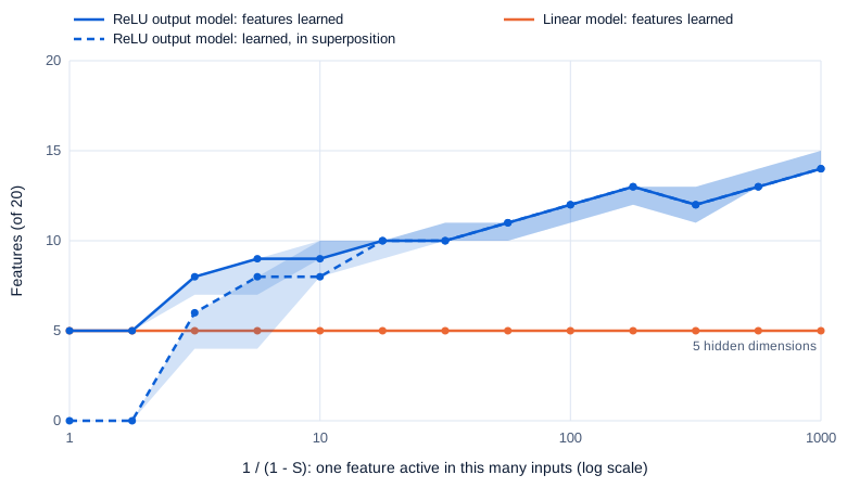
Five numbers can’t hold twenty independent values. Yet a toy network told to try, with features that are each active once in a thousand inputs, keeps 14 of the 20. A linear network of the same size keeps exactly 5, at every sparsity we tried, in all 65 runs.
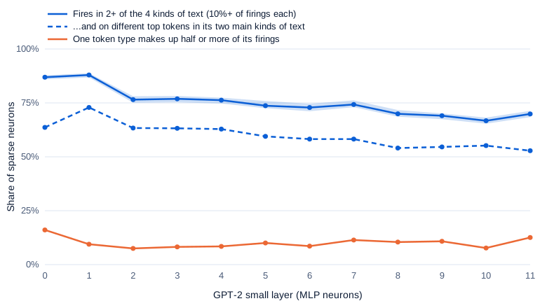
The extra nine live in superposition: their directions overlap, and a ReLU filters out the crosstalk. If real language models do the same, and the evidence below says they do, their neurons can’t be read one at a time. In GPT-2 small, 75% of the MLP neurons that fire rarely split their strongest activations across at least two of four unrelated kinds of text: English web pages, German Wikipedia, Korean Wikipedia and Python code.
Fundamentals Part 16 showed the famous pentagon in one paragraph. This part trains more than 13,000 toy models to measure when superposition appears, what shapes it takes, and how it turns a clean neuron into a messy one.
The intuition
Picture an office with 30 desks and 400 employees who each come in about one day a month. You don’t need 400 desks. Assign several people to each desk, and on most days only one of them turns up. Now and then two desk-mates arrive on the same day and get in each other’s way. That collision is interference.
The arrangement only pays when attendance is rare. If everyone came in daily, you’d give the 30 desks to the 30 most important people and send the rest home, which is exactly what a linear model does.
The analogy breaks in two places. A model’s “desks” are directions, not slots, so two features can share a direction partly, at any angle. And the model has a bouncer: a ReLU (rectified linear unit, which sets negative numbers to zero) at the output, plus a small negative bias, which together throw away weak crosstalk before it reaches the answer.
Step 1: the toy model
Toy Models of Superposition (Elhage et al., 2022) builds the smallest setting where the question has a definite answer. Imagine an ideal, much larger model whose every neuron is one clean feature. The input x is that model’s activations: n numbers, each one a feature. Each feature is 0 with probability S, the sparsity, and otherwise a random value between 0 and 1. The toy network must squeeze x into m hidden numbers, with m smaller than n, and rebuild it.

Both use the same matrix to squeeze and to expand, so each feature has exactly one direction you can point to. Written out:
linear model:       x' = Wᵀ W x + b
ReLU output model:  x' = ReLU(Wᵀ W x + b)
loss = Σ_i I_i (x_i − x'_i)²
W is an m × n matrix whose column W_i is feature i’s direction in the hidden space, b is one bias per feature, and I_i is the feature’s importance, a weight on its error. The product Wᵀ W is an n × n matrix of rank at most m, the kind of thin matrix Math Part 13 took apart with the SVD (singular value decomposition). Its diagonal says how strongly each feature comes back, and its off-diagonal entries are the dot products between feature directions, from Math Part 2: the interference.
For the linear model, Math Part 13’s Eckart-Young theorem settles the outcome. The best rank-m reconstruction keeps the m most important directions and drops the rest, which is principal component analysis (PCA). The paper puts it as “the linear model always learns the top-m most important features, analogous to learning the top principal components.” The ReLU changes the bargain because interference that comes out negative is clipped to zero for free.
Training one on a laptop
The paper’s MIT-licensed notebook trains many small models at once as “instances” of one batched model. This listing does the same for 20 copies of the 5-features-in-2-dimensions model, with every feature active 5% of the time and equal importance. It uses the notebook’s settings (AdamW, learning rate 0.001, batches of 1,024, 10,000 steps) and runs as shown in about 30 seconds on a laptop CPU with PyTorch 2.11:
import torch

torch.manual_seed(0)
n, m, k = 5, 2, 20                    # 5 features, 2 hidden dimensions, 20 models trained at once
density = 0.05                        # each feature is nonzero 5% of the time (sparsity S = 0.95)
W = torch.nn.Parameter(torch.randn(k, n, m) * (2 / (n + m)) ** 0.5)
b = torch.nn.Parameter(torch.zeros(k, n))
opt = torch.optim.AdamW([W, b], lr=1e-3)

def run(x):                            # the ReLU output model: x' = ReLU(W^T W x + b)
    h = torch.einsum("bkf,kfh->bkh", x, W)
    return torch.relu(torch.einsum("bkh,kfh->bkf", h, W) + b)

for step in range(10_000):
    x = torch.rand(1024, k, n) * (torch.rand(1024, k, n) < density)
    loss = ((x - run(x)) ** 2).mean(0).sum(-1)     # one loss per model
    opt.zero_grad(); loss.sum().backward(); opt.step()

with torch.no_grad():                  # 2-D toy models get stuck, so keep the best of 20
    x = torch.rand(100_000, k, n) * (torch.rand(100_000, k, n) < density)
    best = ((x - run(x)) ** 2).mean(0).sum(-1).argmin()
Wb = W[best].detach()
print("feature lengths:", Wb.norm(dim=1).numpy().round(2))
angles = torch.atan2(Wb[:, 1], Wb[:, 0]).rad2deg().sort().values
gaps = torch.cat([angles.diff(), 360 + angles[:1] - angles[-1:]])
print("angles between neighbors:", gaps.numpy().round(1))
print("bias:", b[best].detach().numpy().round(2))
feature lengths: [1.13 1.13 1.13 1.13 1.13]
angles between neighbors: [72. 71.9 72.2 72.1 71.8]
bias: [-0.25 -0.24 -0.25 -0.24 -0.24]Five features in two dimensions, spaced 72 degrees apart: a regular pentagon. Each direction has squared length 1.13² = 1.28, so a lone feature at value 1 comes back as 1.28 − 0.25 = 1.03. A neighbor 72 degrees away leaks 1.28 × cos 72° = 0.39 times its own value into this feature’s output, and the bias of −0.25 cancels that leak unless the neighbor is above 0.63. The two features 144 degrees away leak 1.28 × cos 144° = −1.03 times their value, a negative number the ReLU turns into zero. The cost is that small true values get clipped too: a lone feature below 0.2 comes back as 0.
The rest of this part runs the model at scale with a small module, lab/toy.py, on an NVIDIA GeForce RTX 4060 Laptop GPU (8 GB) in fp32. Every number below comes from models we trained, not from the paper’s figures.
Step 2: when does superposition switch on?
Twenty features, five dimensions
The paper’s first experiment uses 20 features in 5 dimensions with importance falling as 0.7^i, so feature 0 matters most and feature 19 about a thousandth as much. We trained it at 13 sparsity levels, from every feature always active to each active in 1 input of 1,000, with 5 replicates each, for both models. A feature counts as learned if its direction has length at least 0.5, and as in superposition if, in addition, the squared overlaps of the other features with its direction add up to more than 0.1.
Swipe to pan the diagram, or tap it to zoom.
The linear model keeps 5 features at every sparsity, in all 65 runs, and never puts any in superposition. The ReLU model matches it while features are dense, at densities 1 and 0.56. Then it starts packing:
| Feature density (1 − S) | ReLU model: features learned (5 runs) | Of which in superposition | Linear model |
|---|---|---|---|
| 1 and 0.56 | 5 in every run | 0 | 5 |
| 0.32 | 7 to 8 | 4 to 6 | 5 |
| 0.10 | 9 to 10 | 8 to 10 | 5 |
| 0.01 | 11 to 12 | 11 to 12 | 5 |
| 0.001 | 14 to 15 | 14 to 15 | 5 |
By density 0.1, almost every learned feature is in superposition, including the most important ones. The 14th feature kept at the sparsest setting has importance 0.7^13 ≈ 0.01, so the model is now spending space on features that matter a hundredth as much as the first, because sharing is cheap when collisions are rare.
A phase diagram
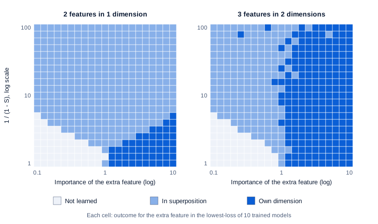
To isolate the effect, the paper shrinks the model to one “extra” feature competing for room. With 2 features in 1 dimension, there are only three things a feature can do: be dropped, get the dimension to itself, or share it with the other feature by pointing the opposite way, an arrangement called an antipodal pair. We varied the extra feature’s importance from 0.1 to 10 times the other’s and the density from 1 to 0.01, on a 21 by 21 grid with 10 models per cell, then did the same with 3 features in 2 dimensions: 8,820 models in all.
Swipe to pan the diagram, or tap it to zoom.
With dense features, the 2-in-1 model behaves like the linear one: the extra feature is dropped if it matters less than the first and takes the dimension if it matters more. As features get sparser, the superposition region spreads out from importance 1, and from 1/(1 − S) of about 6 upward (density 0.16) the extra feature shares the dimension at every importance we tried. The 3-in-2 diagram keeps a large “own dimension” region: an important extra feature gets a dimension to itself while the other two share the second one as an antipodal pair, however sparse the features are.
The boundaries are sharp, which is what the paper means by a phase change: the best arrangement jumps from one solution to another. Training is also hardest there. The paper averaged 9 of its 10 models per point; on our grid, that majority vote agreed with the lowest-loss model in 85% of cells for 2-in-1 and 80% for 3-in-2, and all 10 models agreed in only 54% and 25% of cells. The disagreements are runs stuck in a worse arrangement.
Step 3: the geometry of the packing
Pentagons and pairs, counted
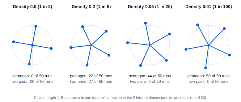
Back to 5 equally important features in 2 dimensions, the paper’s pentagon example, now with 50 training runs at each of 8 densities. The paper warns that two-dimensional models are hard to optimize, so we counted which arrangement each run reached:
Swipe to pan the diagram, or tap it to zoom.
At densities 0.5 and 0.3, the winner is two antipodal pairs at right angles with the fifth feature dropped; 29 and 40 of the 50 runs found it. At 0.2, the two arrangements compete almost evenly, 22 pentagons against 27 pairs, but the best pentagon has the lower loss, 0.078 against 0.082. From 0.05 down, nearly every run makes the pentagon, and at 0.02 and 0.01 all 50 do. Seeing both shapes side by side near the boundary is the paper’s first-order phase change, run by run.
Dimensions per feature, and its sticky fractions
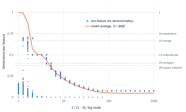
With many features, a number replaces the picture. A feature’s dimensionality is
D_i = ‖W_i‖² / Σ_j (Ŵ_i · W_j)²where Ŵ_i is feature i’s direction scaled to length 1. The top says how strongly the feature is stored, and the bottom how much of its direction it shares, counting itself. A feature with a dimension to itself scores 1, each member of an antipodal pair 1/2, each corner of the pentagon above 2/5, and a dropped feature 0. The average over the model, the paper’s “dimensions per feature”, is m / ‖W‖², the hidden size divided by the total squared length of all the feature directions.
We trained the paper’s large setting, 400 equally important features in 30 dimensions, at 30 densities with 3 replicates each:
Swipe to pan the diagram, or tap it to zoom.
The dimensions-per-feature line is “sticky” at 1 and 1/2, as the paper found. At 1/(1 − S) of 2.6 and 3.3 it sits at 0.51 and 0.50, and every learned feature in all six of those models lies within 0.02 of 1/2: 58 features, 29 antipodal pairs, in 30 dimensions. Just sparser, the features regroup. At 4.2, 24% of learned features sit at 1/2 and 23% at 2/5, pentagons; at 5.3, 48% sit at 3/8, the paper’s square antiprism, and 12% at 2/5. A cluster near 0.7, between the triangle’s 2/3 and the tetrahedron’s 3/4, shows up at 1.3 to 2.
The dimensionalities also always add up to the number of dimensions: across all 90 models, at every sparsity, the sum over 400 features came to between 29.9 and 30.0. The paper noted this holds when features are “packed efficiently”, and here it held every time, so the space is always fully used, just divided differently. Past 1/(1 − S) of about 7, though, our models stop forming the paper’s distinct fractions. All learned features in a model share one value, and that value falls smoothly as more features crowd in, until from about 90 on all 400 features are stored at 0.075 each, which is 30/400. The paper itself suspects the polytope structure is “at least partly idiosyncratic to the toy model”; in our runs it lives in a narrow band of sparsity.
Step 4: from features to neurons
A privileged basis
So far nothing made one hidden direction special. Rotate W and the model is unchanged, the way the residual stream has no preferred axes. Neurons are different: an activation function applied number by number makes the basis directions special, which the paper calls a privileged basis. Its toy for this puts a ReLU on the hidden layer, x' = ReLU(Wᵀ ReLU(W x) + b), so each hidden number is now a neuron, and W says directly which features each neuron carries.
We trained the paper’s setting, 10 features with importance 0.75^i on 5 neurons, at 8 densities with 500 runs each, and counted the features whose weight on a neuron is at least 0.3. A neuron carrying exactly one feature is monosemantic; one carrying two or more is polysemantic.
| Feature density | Features learned (best run of 500) | Monosemantic neurons, best run | Monosemantic neurons, mean of 500 runs |
|---|---|---|---|
| 1 | 5 | 5 of 5 | 4.4 |
| 0.37 | 6 | 3 | 3.2 |
| 0.14 | 7 | 1 | 0.7 |
| 0.05 | 8 | 0 | 0.1 |
| 0.02 and sparser | 10 | 0 | 0.0 |
The counts barely move if the cut-off is 0.2 or 0.4 instead of 0.3. With dense features, every neuron is one feature, the clean case that makes neuron-by-neuron interpretability work. As features get sparser, the model packs more features onto the same 5 neurons, and the neurons become polysemantic, until all 10 features are stored and each neuron carries 7 to 10 of them. That is the paper’s “shift from monosemantic to polysemantic neurons as sparsity increases”, measured. The mixed neurons belong to the lowest-loss runs, so mixing is what the optimizer prefers here.
What GPT-2 small’s neurons look like
If real models do this, an MLP neuron’s strongest activations should come from things that have nothing in common. We ran GPT-2 small (openai-community/gpt2, 124 million parameters, MIT license; fp32, TransformerLens 3.9.0 without weight processing) on 1,600 windows of 127 tokens: 400 each from English web text (FineWeb-Edu held-out documents, ODC-By 1.0), German Wikipedia (53 random articles, CC BY-SA 4.0), Korean Wikipedia (168 random articles and lead sections, CC BY-SA 4.0) and Python code (80 files from the CPython 3.12 standard library, PSF License). That’s 203,200 scored tokens. We read all 36,864 MLP neurons after the GELU, the smooth ReLU-like activation GPT-2 uses (Fundamentals Part 6 builds the MLP).
First, neurons are not a sparse code. On a typical token, 282 to 853 of a layer’s 3,072 neurons are positive, depending on the layer and the kind of text. Only by a strict cut-off do they look selective: say a token fires a neuron when the activation is above half that neuron’s maximum on this sample. Then 34,582 neurons, 94%, fire on at least 20 tokens but fewer than 1% of them.
Of those rarely firing neurons:
| GPT-2 small MLP neurons that fire rarely (34,582) | Share |
|---|---|
| Firings spread over 2 or more of the 4 kinds of text (each with 10% or more) | 75% (74 to 76%) |
| Spread over 3 or more | 29% (28 to 30%) |
| 90% or more of firings in a single kind of text | 20% |
| One token type, such as “per”, is half or more of all firings | 10% |
| Spread over 2+ kinds, on different top tokens in the two main ones, no token type at half | 60% |
The first two intervals are 95% bootstrap intervals over windows; with the four labels shuffled across windows, 99.97% of neurons would count as spread, so the 75% does reflect real domain structure. The share depends on the cut-off: requiring 20% of firings per kind of text instead of 10% gives 52%, and 5% gives 87%. The median rarely firing neuron spreads its firings over 66 token types, the most common one taking 16%.
Swipe to pan the diagram, or tap it to zoom.
Mixing is highest in the first two layers and falls with depth, which fits what Gurnee et al. (2023) found with sparse probes on models from 70 million to 6.9 billion parameters: “early layers make use of sparse combinations of neurons to represent many features in superposition”, while “middle layers have seemingly dedicated neurons to represent higher-level contextual features”.
Spreading across kinds of text isn’t proof of polysemanticity. Neuron 3.924 (layer 3, neuron 924) fires on ” is” in English and on ”=” in Python, arguably one idea. Neuron 8.2426 fires on modal verbs, “to”, “will”, “may”, “can”, in English prose and in the Python files. Others are harder to unify: neuron 7.368 fires on ”(” in English and Python and on compass words like “northern”, “central” and “polar”; neuron 9.2701 fires on “of”, “to” and “but” in English and on “import”, “def” and “from” in code. For a rough number, the author of this article rated 30 rarely firing neurons drawn at random, reading only their top firing tokens in each kind of text: 13 showed one pattern (43%, Wilson interval 27 to 61%), 10 showed two or more unrelated patterns (33%, 19 to 51%), and 7 showed no readable pattern (23%, 12 to 41%). With one rater and no context around the tokens, treat these shares as an illustration.
All of this is correlational in Part 1’s sense: it shows what activates the neurons, and only an intervention could show what they do downstream.
In the real world
- The polysemantic neuron is an old observation. In the image model InceptionV1, neuron 4e:55 “responds to cat faces, fronts of cars, and cat legs”, and in a later layer the network takes a clean car detector and “spreads its car feature over a number of neurons that seem to primarily be doing something else”, mostly dog detectors (Olah et al., 2020). Not reproduced here.
- In a one-layer transformer with a 512-neuron MLP, Bricken et al. (2023) describe a neuron that “responds to a mixture of academic citations, English dialogue, HTTP requests, and Korean text”. When a blinded annotator scored 162 features and neurons with a rubric, “the median neuron scored 0”, meaning no hypothesis at all, while the median sparse-autoencoder feature scored 12. Not reproduced here; Part 7 trains one.
- Superposition also explains a kind of memorization. Henighan et al. (2023) trained the same ReLU output model on finite datasets, with 10,000 features at sparsity 0.999, and found that “overfitting corresponds to storing data points, rather than features, in superposition”, with double descent as the model moves between the two regimes.
- Superposition can also carry computation. The toy paper trained a hidden-ReLU model to compute absolute values of 100 sparse features with only 40 neurons. Hänni et al. (2024) construct networks that compute the AND of every pair of
mfeatures with aboutm^(2/3)neurons, up to log factors, and deep networks of widthdthat emulate circuits of width aboutd^1.5. - Scherlis et al. (2022) recast the trade-off as capacity, the fraction of a dimension each feature gets, the same quantity as
D_iabove. In their toy model the optimal allocation represents the most important features monosemantically, less important ones polysemantically, “and entirely ignore[s] the least important features”. - The toy paper also links superposition to adversarial examples: vulnerability to its attacks rose by more than 3 times as superposition formed, tracking features per dimension. Not reproduced here.
Common misconceptions
- “A model with d dimensions can store at most d features.” Only a linear model is limited that way; it kept 5 of 20 features in 5 dimensions in every run. With one ReLU and sparse features the same size of model kept 14, and the dimensionalities still summed to exactly the 5 (or 30) dimensions available.
- “Superposition is a training failure.” It’s the lower-loss solution. At density 0.2, the pentagon that stores all 5 features beat the two pairs that store 4, 0.078 against 0.082. Polysemantic neurons appeared in the toy because they were the better use of 5 neurons.
- “Superposition happens whenever there’s a shortage of room.” It needs sparsity too. With dense features the ReLU model behaved exactly like the linear one, and the phase diagram’s superposition region only opens as features get rarer.
- “The pentagons and tetrahedra are how real models are organized.” They’re exact solutions in a toy with equal, independent features, and even there they appeared only in a band of sparsity, giving way to one smooth value as features crowded in. Real features vary in importance and are correlated.
- “If a neuron fires on Python and on English, it’s polysemantic.” It might be one feature that occurs in both, like the neuron that fires on ” is” and on ”=”. Polysemanticity is a claim about unrelated meanings, which takes more than counting domains to establish.
Key takeaways
- Superposition means storing more features than dimensions, each as its own direction, and paying with interference where directions overlap.
- A linear model never does it: it keeps the top m features, like PCA. Add one ReLU and make features sparse, and a 5-dimensional toy kept 14 of 20 features.
- The switch is sharp. Phase diagrams show features jumping between dropped, shared and dedicated, and 5 features in 2 dimensions jump from two antipodal pairs to a pentagon as they get rarer.
- The packing is geometric: dimensions per feature stick at 1 and 1/2, single features cluster at 2/5 and 3/8, and the dimensionalities always add up to the number of dimensions.
- When the hidden layer has neurons, superposition makes them polysemantic. In GPT-2 small, three quarters of rarely firing MLP neurons split their strongest activations across unrelated kinds of text, most of all in the first layers.
What’s next
If features hide in superposition across many neurons, reading neurons one at a time is reading the wrong unit. Part 7 trains a sparse autoencoder, a wide dictionary that rewrites each activation as a few active features, on GPT-2 small’s residual stream, measures how much of the model it explains, and explores Google DeepMind’s Gemma Scope features on Gemma 2 2B.
Further reading
- Toy Models of Superposition (Elhage et al., 2022): the paper reproduced here, with the phase diagrams, feature dimensionality, the polytope geometry, privileged bases and computation in superposition.
- toy-models-of-superposition (Anthropic, GitHub): the MIT-licensed notebook whose training setup this article follows.
- Superposition, Memorization, and Double Descent (Henighan et al., 2023): the same toy model on finite data, where data points rather than features go into superposition.
- Towards Monosemanticity: Decomposing Language Models With Dictionary Learning (Bricken et al., 2023): polysemantic neurons in a one-layer transformer, and sparse autoencoder features that score far higher on interpretability.
- Zoom In: An Introduction to Circuits (Olah et al., 2020): the cat-faces-and-car-fronts neuron and the car feature spread across dog neurons.
- Finding Neurons in a Haystack: Case Studies with Sparse Probing (Gurnee et al., 2023): sparse probes that find superposition in early layers of real models up to 6.9 billion parameters.
- Polysemanticity and Capacity in Neural Networks (Scherlis et al., 2022): capacity allocation, and when features end up monosemantic, polysemantic or ignored.
- Mathematical Models of Computation in Superposition (Hänni et al., 2024): constructions for computing many Boolean functions with fewer neurons than features.
- Inside the Black Box: Features, Superposition and Circuits (Fundamentals Part 16): the overview, including random near-orthogonal directions in 768 dimensions.
- Vectors and Dot Products (Math Part 2) and Low Rank and the SVD (Math Part 13): the dot products and low-rank matrices behind interference and
Wᵀ W.