
Inside the Model: Interpretability · Part 3 of 12
Linear Probes: Reading What a Model's Activations Encode
Train one-matrix classifiers on GPT-2 small and Qwen2.5-0.5B to read part of speech and truth from every layer, then check whether the probe did the work.
On this page
TL;DR
A linear probe is a small classifier, one matrix and a bias, trained to read a property such as “this word is a noun” or “this sentence is true” from a model’s internal vectors while the model itself stays frozen. This part trains probes on every layer of GPT-2 small and Qwen2.5-0.5B, for part of speech and for true or false city facts, and measures each result against baselines that never look inside the model. It then runs the checks that keep probing honest: random control labels, linear against nonlinear probes, held-out words and cities, and a rephrased template. You’ll learn to read a probing curve, and why a probe that scores 95% still hasn’t shown that the model uses what it found.
Why it matters
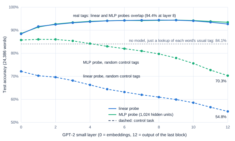
A classifier with 13,073 numbers, reading GPT-2 small’s vector for each word at layer 8, tags parts of speech correctly 94.4% of the time. Give the same classifier random labels instead, a made-up tag for every word, and it still gets 61% of held-out words “right”.
Both numbers come from the run in this article. A probe can report what the model knows, or it can learn the task by itself and take the credit, and telling the two apart decides whether a “truth direction” or a “deception detector” found inside a model means anything.
Fundamentals Part 16 introduced probes in one paragraph, as yes-or-no questions asked of a vector. This part builds them, on two models and two properties, and measures each of the ways they mislead.
The intuition
Guillaume Alain and Yoshua Bengio, who proposed linear probes in 2016, asked readers to “think of those probes as thermometers,” placed at many different locations in the network at once. You push a thermometer into each layer of the network and read off how much of some property is there, without disturbing the model.
The analogy breaks in two ways, and both are the pitfalls of this article. First, a thermometer doesn’t learn. A probe is trained, so a powerful enough probe can work out the answer from raw ingredients the model never combined, like a thermometer that estimates how hot the room is from the color of the walls. Second, a thermometer reading doesn’t tell you the heating system uses that number. A probe shows that information can be read out of a layer, not that any later layer reads it.
Step 1: what a probe is
Take one word in one sentence. After layer 6, GPT-2 small holds a residual stream vector for it: 768 numbers, the running sum that every attention layer and MLP adds to (Fundamentals Part 6 explains the residual stream; Part 2 reads it with the logit lens). A part-of-speech probe turns those 768 numbers into a guess among 17 tags.
A linear probe gives each tag a score by taking a dot product:
score_k = w_k · h + b_k        for each tag k (NOUN, VERB, ADJ, ...)
p(tag k) = softmax(scores)_k
Here h is the 768-number vector, w_k is a learned row of 768 weights for tag k, and b_k is a single learned number, its bias. As Math Part 2 showed, a dot product with a direction measures how far h points along it, so each row is a direction in the model’s space, and the tag whose direction h leans along most wins. The softmax turns the 17 scores into probabilities (Math Part 5).
A toy example with two numbers instead of 768: if h = [2.0, -1.0], the NOUN row is w = [1.5, 0.5] and its bias is -1.0, the NOUN score is 2.0×1.5 + (-1.0)×0.5 - 1.0 = 1.5. If the VERB row scores -0.5, the softmax gives NOUN e^1.5 / (e^1.5 + e^-0.5) = 0.88.
Training means finding the rows and biases that give the gold tag high probability on labeled examples, by minimizing cross-entropy (Math Part 6) with gradient descent. The model’s weights are frozen the whole time; only the probe learns. Here is the whole setup on GPT-2 small, with TransformerLens:
import torch
import transformer_lens as tl

model = tl.HookedTransformer.from_pretrained_no_processing("gpt2", device="cpu")
tokens = model.to_tokens("The old man the boats.")      # prepends <|endoftext|>
_, cache = model.run_with_cache(tokens)
h = cache["blocks.6.hook_resid_pre"][0]                  # layer 6: one 768-number vector per token
print(model.to_str_tokens(tokens), h.shape)

probe = torch.nn.Linear(768, 17)                         # the whole probe: 17 x 768 weights + 17 biases
print(sum(p.numel() for p in probe.parameters()))
scores = probe(h)                                        # one score per tag, for every token
print(scores.shape)                                      # train with cross-entropy against the gold tags
It prints the seven tokens ['<|endoftext|>', 'The', ' old', ' man', ' the', ' boats', '.'], the shape [7, 768], the probe’s 13,073 parameters and the score shape [7, 17]. GPT-2 small has 124 million parameters, so the probe is about one ten-thousandth of its size.

Every box after the frozen model only measures it; turning “readable” into “used” takes an edit to the model itself, which the end of Step 4 previews.
The setup for every number below
All experiments ran on an NVIDIA GeForce RTX 4060 Laptop GPU (8 GB) with TransformerLens 3.9.0 and PyTorch 2.11. GPT-2 small (openai-community/gpt2, 124M parameters, MIT license) ran in 32-bit floats; Qwen2.5-0.5B (Qwen/Qwen2.5-0.5B, Apache-2.0) ran in bfloat16. Both loaded with from_pretrained_no_processing, so LayerNorm was not folded and weights were not centered: “the residual stream” here is the model’s own hidden state, the same numbers Hugging Face returns. “Layer l” means the vector entering block l, so layer 0 is the token embedding plus position and the last layer is the output of the final block, before the final LayerNorm.
Activations were saved to disk once per model, then every probe trained on the saved vectors, each feature rescaled to mean 0 and spread 1 using training statistics. Part-of-speech probes trained with AdamW (learning rate 0.001, weight decay 0.0001) for 10 passes over the data, and the MLP probe has one hidden layer of 1,024 units with a ReLU. Truth probes, with only about 900 training statements per fold, trained for 200 passes with weight decay 0.01, and their MLP probe has 256 hidden units. Collecting both models’ activations took under 3 minutes of GPU time, and all the part-of-speech probes for GPT-2 small took under 4 minutes more; the truth probes, on far less data, trained on the CPU.
Step 2: part of speech, layer by layer
The labels come from Universal Dependencies English EWT v2.18, a corpus of web text (blogs, emails, reviews, forum posts) in which every word carries one of 17 universal part-of-speech tags, from NOUN and VERB to PUNCT and SYM. It is licensed CC BY-SA 4.0. Probes trained on 4,000 randomly chosen training sentences (64,014 words) and were tested on all 2,077 test sentences (24,386 words), so no test sentence was ever seen in training.
GPT-2 splits words into tokens, so a word like “unbelievable” may become several pieces. Each word is read at its last token, which has seen the whole word. GPT-2 reads left to right, so that vector has seen the words before it and none after. Contractions such as “don’t”, which the treebank splits into two syntactic words with no separate spelling, stay in the text but aren’t probed (354 of them in the test set).
Two baselines don’t look inside the model at all. Always guessing NOUN, the most common tag, scores 16.8%. Looking each word up in the training data and guessing its most frequent tag scores 84.1% (95% confidence interval 83.5 to 84.7, from 1,000 bootstrap resamples of test sentences). That lookup is the number to beat, because most English words have one usual part of speech.
| GPT-2 small layer | Linear probe | MLP probe | On words never seen in training |
|---|---|---|---|
| 0 (embeddings) | 88.4% | 88.6% | 71.7% |
| 2 | 92.5% | 92.7% | 80.2% |
| 4 | 93.7% | 93.9% | 84.3% |
| 6 | 94.3% | 94.3% | 86.5% |
| 8 | 94.4% | 94.3% | 86.6% |
| 10 | 94.1% | 94.2% | 86.6% |
| 12 (last block) | 92.7% | 93.4% | 86.0% |
| Word lookup baseline | 84.1% | 34.1% |
Every probe accuracy here has a 95% confidence interval narrower than ±0.4 points, and the last column uses the linear probe.
The embedding layer already beats the lookup, 88.4% against 84.1%, because the probe sees each word’s last token, and endings like “-ly” and “-ing” carry part of speech even for words the lookup has never seen. Accuracy then rises through the first half of the network and peaks at layer 8, as context arrives: “man” in “The old man the boats” is a verb, and only context can say so. The last layers lose a little, plausibly as the vector turns toward predicting the next token.
The strongest evidence comes from words the probe never saw in training, 13.7% of the test set. The lookup gets 34.1% of them, and the linear probe at layer 9 gets 87.2%, which no memorized word list could do.
Qwen2.5-0.5B, with 24 blocks and a different tokenizer, gives the same curve. Its linear probe scores 88.1% at the embeddings, sits between 93% and 94% from layer 3 to layer 20, peaks at 93.9% (93.5 to 94.2) at layer 16, and falls to 91.7% at the last layer. On words never seen in training it reaches 88.7%. A newer model four times the size is no easier to read for part of speech; both plateau near 94%, which may be the most this probe and these labels allow.
Step 3: did the model know it, or did the probe learn it?
John Hewitt and Percy Liang’s Designing and Interpreting Probes with Control Tasks (2019) asked what a probe can do on labels that have nothing to do with language. Their control task gives every word type one random tag, drawn from the real tag frequencies, and keeps it fixed: every “the” might be ADJ and every “cat” PUNCT. The only way to score is to recognize which word each vector came from and memorize its arbitrary tag.
Selectivity is the real accuracy minus the control accuracy. A selective probe does well on the real task and badly on the control, so its success comes from the representation and not its own memory. We ran the control task with three different random seeds on the same words:
Swipe to pan the diagram, or tap it to zoom.
The real-tag lines are almost identical, while the control lines are 14 to 19 points apart: the MLP probe’s extra capacity goes into memorizing.
| GPT-2 small layer | Linear: real | Linear: control | Linear selectivity | MLP: real | MLP: control | MLP selectivity |
|---|---|---|---|---|---|---|
| 0 | 88.4% | 72.2% | 16.2 | 88.6% | 85.8% | 2.8 |
| 4 | 93.7% | 66.3% | 27.4 | 93.9% | 84.2% | 9.7 |
| 8 | 94.4% | 61.0% | 33.4 | 94.3% | 79.7% | 14.6 |
| 12 | 92.7% | 54.8% | 37.9 | 93.4% | 70.3% | 23.2 |
Selectivity is in percentage points, averaged over the three seeds (the seeds differ by under 1 point, and seed 0’s 95% interval at layer 8 for the linear probe is 33.0 to 34.5). The ceiling on the control task is the share of test words seen in training, 86.3%, plus chance on the rest. At layer 0 the MLP probe reaches 85.8%, nearly all of it: given a 1,024-unit hidden layer, it memorized a random tag for almost every word it had seen, and reached 97.6% on its training words.
So the same 94% means different things. The linear probe’s must come mostly from structure in the vectors, while the MLP probe could have reached 80% at layer 8 on memory alone.
This reproduces Hewitt and Liang’s result on a different model. On ELMo, a 2018 recurrent model, their linear probe scored 97.2% on Penn Treebank tags with 71.2% control accuracy, a selectivity of 26.0, while a one-hidden-layer MLP scored 97.3% with 92.8% control, a selectivity of 4.5. They also found that ELMo’s second layer was more selective than its first, though slightly less accurate. GPT-2 small shows the same pattern more strongly: selectivity keeps rising to layer 12, after accuracy has peaked at layer 8, because, as the falling control lines show, later vectors make it harder to tell which word they started as. Qwen2.5-0.5B repeats it: linear selectivity grows from 13.8 at the embeddings to 39.9 at the last layer, and MLP selectivity from 2.3 to 27.0.
Step 4: a probe for truth
Truth is a property of a whole statement, and a truth probe is the kind people want for monitoring. Samuel Marks and Max Tegmark’s The Geometry of Truth (2023) built datasets of simple statements whose truth a model should know, starting with “The city of [city] is in [country].”
We rebuilt that dataset from scratch, from GeoNames (CC BY 4.0), following the paper’s recipe: cities with more than 500,000 people, no name shared with any other city in GeoNames, no city-states. Each city gets one true statement and one false one, and the false country is drawn with probability equal to that country’s share of the true statements, so a statement ending in “China” is not more likely to be true than one ending in “Peru”. We also capped each country at its 40 largest cities and kept countries with at least 3. That leaves 567 cities in 50 countries and 1,134 statements, half true:
The city of Osaka is in Japan.       (true)
The city of Osaka is in Pakistan.    (false)
Each statement is read at its final ”.” token, where Marks and Tegmark found the truth signal in LLaMA-2. Splits are by city: 5-fold cross-validation in which both statements about a city always land in the same fold, so the probe is never tested on a city it trained on. Confidence intervals resample cities.
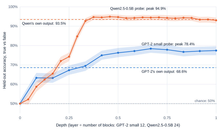
Four baselines frame the result. A bag-of-words classifier, which sees only which words occur, scores 45.1% (42.3 to 48.0): below chance, because the matched sampling leaves it nothing to learn and it overfits to noise. A probe trained on shuffled labels scores 49 to 52% at every layer. The model’s own output is the serious baseline: we scored each statement by the log-probability the model gives the country after “The city of X is in”, and fit a threshold in the same folds. That gets 68.6% for GPT-2 small and 93.5% for Qwen2.5-0.5B. Asked to choose between the true and false country for the same city, GPT-2 small prefers the right one for 75.8% of the cities, and Qwen for 96.5%.
Swipe to pan the diagram, or tap it to zoom.
In both models the probe rises from chance at the embeddings to a plateau, and the plateau sits close to what the model’s own output knows. Qwen2.5-0.5B’s jump between layers 6 and 8 (74.3% to 92.7%) is where it looks the fact up.
The plateau heights follow each model’s knowledge. GPT-2 small’s best linear probe reaches 78.4% (76.3 to 80.5) at layer 8, and Qwen’s reaches 94.9% (93.4 to 96.1) at layer 11. Split by whether the model itself prefers the true country, GPT-2’s layer-8 probe scores 82.0% on the 430 cities it “knows” and 67.2% on the 137 it doesn’t. The probe does best where the model knows the answer, although 67.2% on the rest is above chance.
GPT-2 small’s probe already scores 63.3% after a single block, at layer 1. A linear probe can’t check whether a city matches a country from separate “Osaka” and “Pakistan” features; that match is like an exclusive-or, which no single line can draw. So something in the first block must already combine them, plausibly the MLP acting as a lookup table of common pairs. The MLP probe gains most where the model has computed least: at layer 1 in Qwen, 62.3% against the linear probe’s 52.2%.
Change the sentence, keep the fact
A probe that has found truth should not care how the fact is phrased. We tested the same probes, trained on “The city of X is in Y.”, on the same held-out cities written as “X is a city in Y.” The accuracy fell hard: from 78.4% to 59.1% for GPT-2 small at layer 8, and from 94.7% to 68.8% for Qwen at layer 9. No Qwen layer scored above 73% on the new template.
Much of the drop comes from a moved threshold. Scoring each statement by its projection on the mass-mean direction (the mean true vector minus the mean false vector), which needs no threshold, the AUROC on the new template is 0.94 for Qwen at layer 9, against 0.98 on the original. AUROC is the chance that a random true statement scores higher than a random false one, so 0.5 is chance and 1 is perfect. For GPT-2 small it drops from 0.73 to 0.60. Qwen’s truth direction mostly carries over and only the probe’s cut-off point shifts, while GPT-2’s direction was partly about the template.
A preview of Part 9: push along the direction
To test whether Qwen2.5-0.5B uses its truth direction, we borrowed Marks and Tegmark’s causal test. The model sees four labeled examples (“The city of Paris is in France. This statement is: TRUE”, and three more, two of them false), then a new statement followed by “This statement is:”, and we compare its probabilities of ” TRUE” and ” FALSE”. Unedited, Qwen labels 78.0% of the 1,134 statements correctly (75.7 to 79.9). GPT-2 small scores 49.6%, chance, so it can’t take this test.
Then we edit one vector. At one layer, at the statement’s final ”.”, we add the mass-mean direction to false statements and subtract it from true ones, using a direction computed from the other folds’ cities. The normalized indirect effect, Marks and Tegmark’s measure, is 0 if the answer doesn’t move and 1 if false statements now get as much “TRUE” as real true statements do:
| Qwen2.5-0.5B layer | Direction added | False pushed to true | True pushed to false |
|---|---|---|---|
| 11 | Mass-mean, from the few-shot prompts | 0.11 | 0.16 |
| 13 | Mass-mean, from the few-shot prompts | 0.52 (0.49 to 0.56) | 0.61 (0.58 to 0.65) |
| 13 | The same, 3 times as long | 1.29 | 1.46 |
| 13 | Mass-mean, from Step 4’s statements on their own | 0.34 (0.32 to 0.36) | 0.39 (0.37 to 0.41) |
| 13 | Random, 3 times the mass-mean length | 0.09 | 0.01 |
| 15 | Mass-mean, from the few-shot prompts | 0.03 | 0.03 |
Intervals resample cities. At layer 13 the direction is about an eighth of the vector’s length, and adding it moves the model’s verdict about halfway; three times as much overshoots, making false statements look truer than true ones. A random direction three times as long barely moves it.
The layers matter most. A probe reads truth at 93 to 95% from layer 8 to the last layer, yet the edit works mainly at layers 13 and 14. By layer 15 the later tokens have presumably already copied what they need from the ”.”, so changing it there does nothing. This is one token at one layer; Part 9 covers steering properly.
In the real world
- Marks and Tegmark found that “at sufficient scale, LLMs linearly represent the truth or falsehood of factual statements” in LLaMA-2-13B and 70B (not reproduced here). Probes trained on cities transferred to other kinds of true and false statements better in larger models, and simple mass-mean probes generalized about as well as logistic regression. Adding the mass-mean direction made LLaMA-2-13B label false Spanish-translation statements as true with a normalized effect of 0.77, against 0.13 for the logistic-regression direction.
- Wes Gurnee and Max Tegmark’s Language Models Represent Space and Time (2023) trained linear probes on the Llama-2 family and found linear representations of places’ coordinates and of when events happened, robust to prompt changes and shared across cities and landmarks (not reproduced here).
- Anthropic’s Simple probes can catch sleeper agents (MacDiarmid et al., April 2024) built a linear detector from a single contrast pair, “Human: Are you a helpful AI? Assistant: no” against the same with “yes”, and used it on the middle residual stream of models trained to write vulnerable code when triggered. It flagged the triggered prompts with an AUROC of 99.3% (not reproduced here).
- Google DeepMind’s interpretability team found linear probes beat sparse autoencoders at detecting harmful intent in prompts, as Fundamentals Part 16 described.
- Yonatan Belinkov’s review of probing classifiers (2021) collects the caveats, and Amnesic Probing (Elazar et al., 2021) tested them on BERT: removing a property that probes read well did not always hurt the task, so “conventional probing performance is not correlated to task importance.”
Common misconceptions
- “High probe accuracy means the model uses that information.” A probe measures what a later layer could read, not what any layer does read. Only an intervention, like the nudge above or the patching in Part 5, tests use.
- “A more powerful probe gives a truer picture.” The MLP probe matched the linear one on real tags and beat it on random ones by up to 19 points. Extra power mostly bought memorization.
- “If accuracy peaks at a layer, the property lives there.” Accuracy peaked at layer 8 for part of speech, but selectivity kept rising to layer 12. Which layer “represents” a property depends on the measure you choose.
- “A truth probe detects truth.” Ours tracked what each model knows, fell from 94.7% to 68.8% when the sentence was rephrased, and couldn’t separate truth from closely related things like “commonly believed” or “likely text”, a limit Marks and Tegmark state for their own datasets.
- “Random splits are good enough.” If the same city or the same sentence lands on both sides of the split, a probe can score by remembering it. Every split here was by sentence or by city.
Key takeaways
- A linear probe is one matrix trained on a frozen model’s vectors. It reads a property as a direction, so it asks a precise question: is this information linearly readable at this layer?
- On GPT-2 small, part of speech peaks at 94.4% at layer 8, ten points above a word lookup, and reaches 87% on words the probe never saw.
- Control tasks keep probes honest. With random tags, the linear probe fell to 61% at layer 8 while an MLP probe held 80%, so the same accuracy can mean structure or memory.
- Truth probes rise to roughly what the model’s own output already knows: 78% for GPT-2 small and 95% for Qwen2.5-0.5B on the same 1,134 city statements, with nothing learned from the cities in the test folds.
- A readable direction isn’t automatically a used one. Qwen’s truth direction was readable from layer 8 to the end, but pushing along it changed the model’s answer mainly at layers 13 and 14.
What’s next
Probes read what a layer holds. Part 4 looks at the machinery that moves information between tokens in the first place: attention heads. It finds GPT-2 small’s induction heads, the heads that spot a repeated pattern and copy what came next, measures how they let the model learn from its own prompt, and knocks them out to see what breaks.
Further reading
- Understanding intermediate layers using linear classifier probes (Alain & Bengio, 2016): the paper that named probes, with the thermometer analogy and per-layer probes on Inception v3 and ResNet-50.
- Designing and Interpreting Probes with Control Tasks (Hewitt & Liang, 2019): control tasks and selectivity, with linear and MLP probes on ELMo.
- The Geometry of Truth: Emergent Linear Structure in LLM Representations of True/False Datasets (Marks & Tegmark, 2023): the cities dataset, mass-mean probes and causal interventions on LLaMA-2.
- Probing Classifiers: Promises, Shortcomings, and Advances (Belinkov, 2021): a review of what probes can and can’t show.
- Amnesic Probing: Behavioral Explanation with Amnesic Counterfactuals (Elazar et al., 2021): removing a property to test whether the model uses it.
- Language Models Represent Space and Time (Gurnee & Tegmark, 2023): linear probes for coordinates and dates in Llama-2.
- Simple probes can catch sleeper agents (Anthropic, 2024): a one-pair linear detector for backdoored behavior.
- UD English EWT (Universal Dependencies): the part-of-speech treebank used here, CC BY-SA 4.0.
- GeoNames data export: the city list behind the truth dataset, CC BY 4.0.
- TransformerLens: the library used to cache and edit activations.