
Inside the Model: Interpretability · Part 8 of 12
Circuits and Attribution Graphs, Traced on a Laptop GPU
From hand-found circuits to attribution patching, transcoders and attribution graphs, run with circuit-tracer on Gemma 2 2B and tested by intervention.
On this page
TL;DR
A circuit is the part of a model that carries out one behavior, written as a small graph of components and the connections between them. The first ones were found by hand. This part follows the automation: attribution patching replaces thousands of patching runs with one backward pass, transcoders replace the dense MLPs with sparse, readable features, and attribution graphs combine the two into a map of which features pushed which on one prompt. We ran the open-source circuit-tracer library on Gemma 2 2B on an 8 GB laptop GPU, built graphs for three prompts, and tested them by editing the model. You’ll see what the graphs get right, what they leave unexplained, and why each one is a hypothesis until an intervention confirms it.
Why it matters
Ask Gemma 2 2B to finish “Fact: the capital of the state containing Dallas is” and it says ” Austin”, with 41% probability. Nothing in the prompt says “Texas”. To get it right, the model has to work out the state and then that state’s capital.
An attribution graph built for this prompt on a laptop, in 12 seconds, points to a handful of features on the word “Dallas” that circuit-tracer’s authors label “Texas”. Suppress those six features and the chance of ” Austin” falls from 41% to 0.00%, and other state capitals, ” Albany” and ” Hartford”, rise to the top of the list. Suppress them and add five features taken from a prompt about Oakland, and the model answers ” Sacramento” at 27%.
So the graph found a real step inside the model. It also leaves a lot unexplained: its transcoders miss 42% of the variance of a typical MLP’s output, and when we removed 150 graph nodes one at a time, the graph’s own ranking predicted the effects only weakly. This part shows both results.
The intuition
Picture an unlabeled electrical board, and a lamp that turns on when you flip one switch. To find out why, you could cut wires one at a time and watch the lamp, which is slow. Or you could measure the current in every wire once, with the switch on, and draw a diagram of which wires carry the most current toward the lamp.
An attribution graph is that diagram. To draw it, you first swap the board’s tangled custom chips for standard parts whose behavior you can read off: those are the transcoders. Wherever a standard part doesn’t match the chip it replaced, you put a box labeled “unexplained” on the diagram, so the totals still add up. Those boxes are the error nodes.
The analogy breaks in two places. A model’s “wires” are directions in vectors, and many signals share each one. And the diagram is drawn for one setting of the switches: attention patterns, which decide where each token looks, are frozen at their values on this one prompt, so the diagram can’t show why the model looked where it did.
Step 1: from hand-found circuits to automated discovery
The best-known hand-found circuit is the one for indirect object identification (IOI) in GPT-2 small (Wang et al., 2022). Given “When Mary and John went to the store, John gave a drink to”, the model should say ” Mary”, the name that appeared once. The authors found 26 attention heads in 7 classes, including name mover heads that copy the right name and S-inhibition heads that tell them not to copy the repeated one. Part 5 covered their tool, activation patching: paste one activation from a clean run into a corrupted run and see how much of the right answer comes back.
Patching is expensive: one forward pass per component, or per connection. Conmy et al. (2023) automated it with ACDC (Automatic Circuit DisCovery), which walks the model’s graph of components and deletes every connection whose removal barely changes the output. It “rediscovered 5/5 of the component types” of a known circuit in GPT-2 small and “selected 68 of the 32,000 edges”, all of which earlier hand analysis had found. But it still needs a forward pass per test.
Attribution patching, from a 2023 post by Neel Nanda, replaces those passes with calculus. Run the corrupted prompt once forward and once backward, and you have the gradient of the metric with respect to every activation. A first-order estimate of patching any activation is then one multiplication:
estimated effect ≈ (clean activation − corrupted activation) · gradient at the corrupted runThe metric is the logit difference: the model’s score for ” Mary” minus its score for ” John”. If the clean activation of a head differs from the corrupted one by a vector Δ, and the metric changes by g per unit along each direction, the estimate is the dot product Δ · g. Two forward passes and one backward pass give it for every head, every layer and every position at once. Syed et al. (2023) applied this to every edge, calling it edge attribution patching, and found it competitive with ACDC “while requiring just two forward passes and a backward pass”.
Measured: how good is the estimate?
We built 120 IOI prompts for GPT-2 small from 3 templates (“When A and B went to the [place], B gave a [object] to”, and two variants), with 30 single-token names, both name orders, and 40 prompts per template. The corrupted prompt flips the second mention of the subject to the other name, so the right answer flips too. The clean logit difference averages 3.35 and the corrupted one -3.12. GPT-2 small ran in fp32 through TransformerLens 3.9.0 with weight processing on, on an NVIDIA GeForce RTX 4060 Laptop GPU (8 GB).
This listing runs as shown and does the whole method on one prompt pair:
import torch
from transformer_lens import HookedTransformer

model = HookedTransformer.from_pretrained("gpt2", device="cuda")  # fp32, LayerNorm folded
clean = model.to_tokens("When Mary and John went to the store, John gave a drink to")
corr = model.to_tokens("When Mary and John went to the store, Mary gave a drink to")
mary, john = model.to_single_token(" Mary"), model.to_single_token(" John")
ld = lambda logits: logits[0, -1, mary] - logits[0, -1, john]   # logit difference

_, clean_cache = model.run_with_cache(clean)
acts, grads = {}, {}
for l in range(12):                                  # cache z and its gradient on the corrupted run
    model.add_hook(f"blocks.{l}.attn.hook_z", lambda x, hook: acts.__setitem__(hook.name, x.detach()))
    model.add_hook(f"blocks.{l}.attn.hook_z", lambda g, hook: grads.__setitem__(hook.name, g.detach()), dir="bwd")
corr_ld = ld(model(corr))
corr_ld.backward()
model.reset_hooks()

# Attribution patching: (clean - corrupted) x gradient, for all 144 heads at once
est = torch.stack([((clean_cache[n] - acts[n]) * grads[n]).sum((0, 1, 3)) for n in sorted(acts, key=lambda n: int(n.split(".")[1]))])
print("logit difference, clean", round(ld(model(clean)).item(), 2), "corrupted", round(corr_ld.item(), 2))
for i in est.flatten().abs().argsort(descending=True)[:4].tolist():
    l, h = divmod(i, 12)
    def patch(z, hook): z[:, :, h] = clean_cache[hook.name][:, :, h]; return z
    with torch.no_grad():
        true = ld(model.run_with_hooks(corr, fwd_hooks=[(f"blocks.{l}.attn.hook_z", patch)])) - corr_ld
    print(f"head {l}.{h}: estimate {est[l, h]:+.2f}, true patch {true.item():+.2f}")
It prints (TransformerLens also warns on stderr that from_pretrained is deprecated):
Loaded pretrained model gpt2 into HookedTransformer
logit difference, clean 3.36 corrupted -2.48
head 10.7: estimate -2.35, true patch -2.69
head 9.9: estimate +1.76, true patch +1.43
head 8.10: estimate +1.50, true patch +1.48
head 8.6: estimate +1.43, true patch +1.28
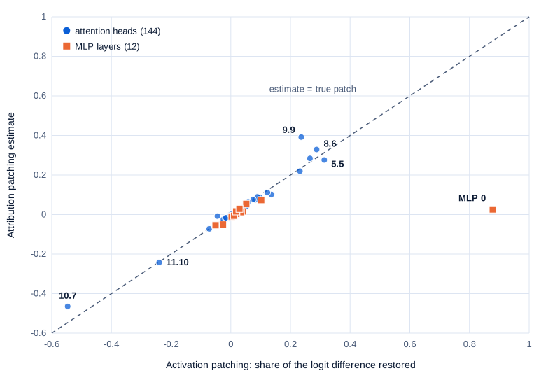
hook_z is each head’s output before the output matrix. On all 120 prompts we compared the estimate with real activation patching for every head (144 patches), every attention and MLP layer (12 each) and the residual stream at every layer and position (180), each as the share of the clean-minus-corrupted gap that the patch restores:
| Component (GPT-2 small, 120 IOI prompts) | Correlation of estimate with true patch (95% CI) | Notes |
|---|---|---|
| Attention heads, 144 | 0.976 (0.972 to 0.979) | 9 of the top 10 heads agree |
| Attention layer outputs, 12 | 0.97 (0.97 to 0.98) | |
| Residual stream, layer by position, 180 | 0.75 (0.71 to 0.78) | Layer 0 at the repeated name: true 1.00, estimate 0.01 |
| MLP layer outputs, 12 | 0.29 (0.06 to 0.48) | MLP 0: true 0.88, estimate 0.03 |
Intervals come from 1,000 bootstrap resamples of prompts. The real patches took 1,056 forward passes and 42.5 seconds; the estimates took 0.86 seconds, 49 times faster, and the gap grows with the number of components.
Swipe to pan the diagram, or tap it to zoom.
The top heads by both methods belong to Wang et al.’s classes: name mover 9.9, S-inhibition heads 7.3, 7.9, 8.6 and 8.10, induction head 5.5 (from Part 4) and duplicate-token head 3.0, plus the negative name movers 10.7 and 11.10, which push against the right answer.
The failures are where Nanda predicted, that the method “works badly for residual streams and MLP0, well for everything else”. Patching MLP 0 or the whole residual stream at the repeated name swaps in a large chunk of the token’s representation. A linear estimate only holds for small changes. So attribution patching is a good screen for where to look, and the big effects it flags, or misses, still need a real patch.
Step 2: transcoders, a readable stand-in for the MLPs
MLPs are the harder part. Each GPT-2 MLP has 3,072 neurons, and as Part 6 showed, neurons are polysemantic: one neuron responds to many unrelated things. A circuit drawn through neurons is enormous or unreadable.
Part 7 used sparse autoencoders (SAEs) to rewrite an activation as a few active features. A transcoder does the same job for a whole MLP (Dunefsky et al., 2024). It reads the MLP’s input and is trained to predict the MLP’s output through a wide, sparse layer of features:
f = JumpReLU(W_enc x + b_enc)      a few thousand candidate features, almost all exactly 0
ŷ = W_dec f + b_dec                predicted MLP output
JumpReLU sets a feature to 0 unless its input passes a learned threshold (Rajamanoharan et al., 2024). The swap simplifies connections. Between two transcoder features, in layers l and l', the contribution of the first to the second on a token factors into one number that depends on the input, the first feature’s activation, and one that doesn’t: the dot product of its decoder vector with the second feature’s encoder vector. Dunefsky et al. call the second term input-invariant: “once the transcoders have been trained, this term does not depend on the input to the model.”
A cross-layer transcoder (CLT), the variant Anthropic uses, lets each feature read from one layer and write to the MLP outputs of every later layer. One feature can then stand in for a chain of similar features in successive layers, which shortens the paths a person has to read.
Measured: how much of each MLP do the transcoders capture?
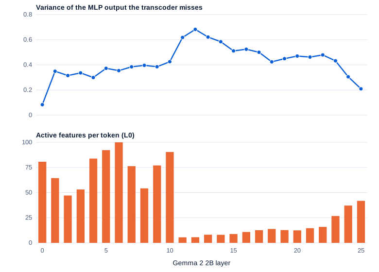
Google DeepMind’s Gemma Scope released one suite of single-layer transcoders for Gemma 2 2B (google/gemma-scope-2b-pt-transcoders, CC-BY-4.0), 16,384 features per layer. circuit-tracer’s Gemma configuration uses the sparsest one for each of the 26 layers. We downloaded those 26 files (7.9 GB of float32), converted them to 3.9 GB of bf16, and measured them on 8,192 tokens: 64 held-out FineWeb-Edu documents (ODC-By) of 128 tokens.
Gemma 2 2B (google/gemma-2-2b, 2.6 billion parameters, Gemma Terms of Use) ran in bf16 on the GPU without TransformerLens weight processing. The fraction of variance unexplained (FVU) is the squared error of the transcoder’s prediction divided by the variance of the true MLP output: 0 is perfect, 1 is no better than predicting the average.
Swipe to pan the diagram, or tap it to zoom.
Layers 11 to 14 use 5.5 to 8 active features per token and miss 58% to 68% of the variance; across all 26 layers the average miss is 42%. This suite trades accuracy for sparsity, so the graphs built on it stay small enough to read. The Gemma Scope paper itself reports that its transcoders “cause a greater increase in loss to the base model” than its MLP-output SAEs at the same sparsity.
The transcoders expect the MLP’s input after the RMSNorm’s division but before its learned gain, which Gemma Scope folded into the MLP weights. Fed that, layer 0 misses 8% of the variance with 81 features per token, close to the 76 in its file name; fed the input after the gain, it misses 1,250%.
Errors compound when every MLP is swapped at once. With all 26 replaced, the next-token loss rose from 2.62 nats (2.51 to 2.74) to 5.51 (5.31 to 5.71), and the replacement model’s top token matched the real model’s on 33.9% of tokens (32.5 to 35.2%). On the tokens Anthropic uses for this test, ones the model gets right with under 80% confidence, the match was 33.6% of 2,403. For comparison, Anthropic’s largest CLT on its own 18-layer model “matches the underlying model’s next-token completion on 50%” of such prompts; that’s a different model and a better transcoder type, not reproduced here.
Step 3: attribution graphs
A replacement model that gets two-thirds of its top tokens wrong can’t explain the real one. Ameisen et al. (2025) fix this per prompt with a local replacement model. It swaps the MLPs for transcoders, freezes the attention patterns and normalization denominators at their values on this prompt, and adds an error term at every layer and position: the true MLP output minus the transcoder’s. The activations and output now match the real model exactly, and what’s left between features is linear.
So the effect of one node on another is a single number, and the graph is a matrix of them. Its nodes are the input tokens, every active feature at every position, one error node per layer and position, and the top output tokens. One backward pass per node, run in batches, fills in all the edges.

Everything before the last box happens inside the replacement model; only the last box touches the real one.
Two scores say how much of a graph is explained, both computed before pruning. The replacement score is the share of influence from input tokens to the output that flows through features instead of error nodes. The completeness score is gentler: for each node it asks what fraction of its input comes from features or tokens, weighted by how much that node matters. Pruning then keeps the smallest set of nodes that carries 80% of the influence on the output, and the edges that carry 98%.
Running circuit-tracer on 8 GB
circuit-tracer (MIT license, version 0.5.0) is the library Anthropic’s Fellows built with Decode Research and open-sourced in May 2025. It supports Gemma 2 2B, Llama 3.2 1B, Qwen3 and Gemma 3, and its README points to Colab’s 15 GB GPUs for Gemma 2 2B. Fitting it into 8 GB took four changes:
- circuit-tracer pins
transformersat or below 4.57.3, so it got its own Python environment (with transformer-lens 3.2.1 and torch 2.11), leaving the shared one untouched. - Its loader calls TransformerLens’s standard loader, which builds the whole model in CPU memory first; a test of that loader with Gemma 2 2B on this machine was killed at an 8 GB host-memory cap. We built the model directly on the GPU and copied the weights in one tensor at a time, which kept host memory at 4.9 GB.
- The transcoders in bf16 (3.9 GB) don’t fit next to the model, which takes 6.0 GB on the GPU because TransformerLens keeps separate input and output embedding matrices. circuit-tracer’s lazy loading keeps the transcoder matrices on disk and reads each one only when needed.
- Attribution ran in batches of 64 backward passes, with at most 8,192 feature nodes per graph.
| Prompt (Gemma 2 2B) | Top output | Active features | Feature nodes after pruning | Replacement score | Completeness score | Graph time |
|---|---|---|---|---|---|---|
| Fact: the capital of the state containing Dallas is | ” Austin” (41%) | 9,161 | 1,847 | 0.72 | 0.93 | 12 s |
| The Brandenburg Gate is located in the city of | ” Berlin” (96%) | 7,908 | 1,507 | 0.70 | 0.93 | 7 s |
| When Mary and John went to the store, John gave a drink to | ” Mary” (27%) | 11,622 | 2,076 | 0.74 | 0.93 | 16 s |
The Brandenburg Gate prompt is one of Part 1’s landmark prompts. Graph time excludes the 14 seconds to load the model; peak GPU memory was 7.1 GB for every graph. The Dallas and IOI graphs hit the 8,192-node cap, so they keep the most influential 8,192 features. The Dallas graph also has 286 error nodes, one per layer and position, of which pruning keeps 167.
Anthropic’s per-layer-transcoder example graph scored 0.78 for completeness and 0.37 for replacement, against 0.80 and 0.61 with a CLT on the same prompt. Our higher replacement scores reflect a different model and much shorter prompts, so they don’t show a better method.
The Dallas graph recovers the structure the method’s authors describe. Among its 25 most influential features are five of the six that circuit-tracer’s Gemma demo groups as “Texas”, on the “Dallas” token in layers 4 to 20, plus its “say a capital” feature (layer 21) and its “say Austin” feature (layer 23) on the last token. Direct edges into the ” Austin” output come from the layer-20 Texas feature at the last position (+5.1), the “say a capital” feature (+3.1) and “say Austin” (+2.7). The embedding of “Dallas” itself has a direct edge of +5.0, a shortcut that skips the Texas step, like the “shortcut” edge from Dallas to “say Austin” that Lindsey et al. (2025) found in Claude 3.5 Haiku. Error nodes supply 17% of the absolute weight flowing into the ” Austin” output.
Step 4: testing the graph on the real model
A graph describes the local replacement model. The test is to edit the real model as the graph suggests, with attention free to change, and see if the output moves as predicted.
The Texas swap
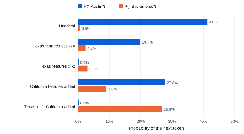
We used the feature lists from circuit-tracer’s demo: six “Texas” features on the Dallas prompt, and five “California” features read from “Fact: the capital of the state containing Oakland is”, which Gemma completes with ” Sacramento” (36%). Each edit adds a feature’s decoder vector to its layer’s MLP output, scaled so the feature reaches the chosen value.
Swipe to pan the diagram, or tap it to zoom.
Setting the Texas features to 0 halves the chance of ” Austin”. Pushing them to minus twice their value removes it, and after ” the” the top guesses are other state capitals: ” Albany”, ” Hartford”. Adding California alone isn’t enough, because Texas still wins. Doing both makes ” Sacramento” the top token at 26.8%. With attention frozen at its original pattern, the swap gives Sacramento 35.9%, so on this prompt the frozen-attention view of the graph is close to the real model.
As a control, we pushed six random active features at the same layers and positions to minus twice their value. That left ” Austin” at a median of 39% over 20 draws, but 7 of the 20 draws pushed it below 20%, and 2 below 1%. Large negative edits to whatever is active can break a prediction by brute force, but the random edits never brought up other state capitals or Sacramento.
Node by node
Anthropic reports that a node’s influence score predicts the effect of ablating it better than its direct edge to the output or its activation does. To test that, we took each graph’s 50 most influential feature nodes, set each to 0 in the real model, and measured how far the top output’s logit moved.
| Rank correlation with the real ablation effect | Dallas (50 nodes) | Brandenburg Gate (50) | IOI (50) | Pooled (150) |
|---|---|---|---|---|
| Graph influence score | 0.50 (0.23 to 0.71) | 0.35 (0.03 to 0.60) | 0.17 (-0.14 to 0.45) | 0.29 (0.12 to 0.43) |
| Direct edge to the output | 0.70 (0.53 to 0.83) | 0.23 (-0.05 to 0.48) | 0.32 (0.04 to 0.55) | 0.41 (0.26 to 0.54) |
| Activation size | 0.33 (0.07 to 0.54) | 0.17 (-0.15 to 0.44) | 0.40 (0.17 to 0.59) | 0.28 (0.13 to 0.42) |
| Same ablation with attention frozen (correlation of effects) | 0.98 | 0.95 | 0.67 | 0.89 |
Intervals are 2,000 bootstrap resamples of nodes. With per-layer transcoders on Gemma 2 2B, the influence score did not beat the simpler baselines; Anthropic’s result is for its CLTs and models and is not reproduced here. The last row shows one reason: on the IOI prompt, ablations with attention frozen agree with the real ones at only 0.67, against 0.95 to 0.98 on the two factual prompts. IOI is an attention circuit: its whole mechanism is which name the heads attend to, and the graph freezes exactly that. Ameisen et al. name this limitation “missing attention circuits”, and write that in some cases it “renders our attribution graphs essentially useless.”
Single-feature ablations are also small (median 0.37 logits), so error nodes and nonlinearities weigh heavily. Groups of related features, like the six Texas features, give large, clean effects, which is why published case studies intervene on supernodes, groups of features with a shared role.
In the real world
- Anthropic’s Circuit Tracing trained CLTs of up to 10 million features on an 18-layer model and 30 million on Claude 3.5 Haiku; the largest Haiku CLT had a normalized reconstruction error of 21.7% with 235 active features per token. Pruning cut graphs by “an order of magnitude while reducing completeness by only 20%.” Feature-to-feature influence had a Spearman correlation of 0.72 with ablation effects. Not reproduced here.
- On the Biology of a Large Language Model applied the graphs to Claude 3.5 Haiku: the Dallas-to-Texas-to-Austin step, rhyme planning, refusals and hallucinations. The authors write that the graphs give “satisfying insight for about a quarter of the prompts we’ve tried.” Not reproduced here.
- The methods paper shows a failure: on an obfuscated jailbreak prompt, “almost all the nodes on the obfuscated prompt tokens are error nodes”, so the origin of the refusal can’t be traced.
- circuit-tracer’s README lists cross-layer transcoders for Gemma 2 2B with 426,000 and 2.5 million features. The smaller set is 33 GB on disk, so we used the per-layer set. Neuronpedia hosts these graphs for browsing and steering online.
Common misconceptions
- “An attribution graph shows how the model computed its answer.” It shows how a local replacement model, with frozen attention and error nodes, computed it. On our three prompts 26% to 30% of the input-to-output influence ran through error nodes, and attention, which carries the IOI mechanism, isn’t explained at all.
- “Attribution patching is just a faster activation patching.” It’s a linear estimate. On IOI heads it matched real patching at a correlation of 0.976, but it estimated MLP 0’s effect at 0.03 when the real patch restored 0.88 of the answer.
- “A high completeness score means the graph is right.” Our graphs scored 0.93, yet single-node ablations agreed with the graph’s ranking only weakly. Completeness counts how much input comes from features, not whether the features act as the graph says.
- “If editing features changes the answer, the graph is confirmed.” Strong negative edits to random features also broke the Dallas answer in 7 of 20 draws. The test is a specific change, like other capitals or Sacramento appearing, compared against controls.
- “Transcoders are a lossless swap for the MLPs.” The Gemma Scope suite used here misses 42% of the variance of the average layer’s MLP output, and swapping all 26 MLPs drops top-token agreement to 34%.
Key takeaways
- Circuits used to be found one patching run at a time. Attribution patching estimates every patch from one backward pass: on GPT-2 small’s IOI task it was 49 times faster and matched real patching on heads at 0.976, but it badly missed the big effects of MLP 0 and the early residual stream.
- Transcoders replace each MLP with sparse, readable features, so connections between features factor into an activation times a fixed weight. The sparse Gemma Scope set on Gemma 2 2B uses 5 to 100 features per token and misses 42% of an average MLP’s variance.
- An attribution graph freezes attention, adds error nodes so the totals match the real model, and measures every direct effect. With circuit-tracer, a graph for Gemma 2 2B took 7 to 16 seconds and 7.1 GB on a laptop GPU.
- The Dallas graph found the Texas step. Editing six Texas features and five California features turned ” Austin” at 41% into ” Sacramento” at 27%.
- Graphs are hypotheses. Single-node predictions were weak, attention-driven behavior like IOI is largely invisible, and every claim needs an intervention and a control on the real model.
What’s next
Swapping Texas for California was a small act of steering, done through features a graph pointed to. Part 9 makes steering the subject: adding directions to the residual stream to change what a model does, finding the single direction that controls refusal, and measuring what else breaks when you push.
Further reading
- Circuit Tracing: Revealing Computational Graphs in Language Models (Ameisen et al., 2025): cross-layer transcoders, the local replacement model, error nodes, pruning, replacement and completeness scores, and the method’s limitations.
- On the Biology of a Large Language Model (Lindsey et al., 2025): attribution graphs on Claude 3.5 Haiku, including the Dallas two-hop example.
- Transcoders Find Interpretable LLM Feature Circuits (Dunefsky, Chlenski & Nanda, 2024): transcoders and the input-invariant factorization of feature-to-feature connections.
- Towards Automated Circuit Discovery for Mechanistic Interpretability (Conmy et al., 2023): ACDC.
- Attribution Patching Outperforms Automated Circuit Discovery (Syed, Rager & Conmy, 2023): edge attribution patching.
- Attribution Patching: Activation Patching At Industrial Scale (Nanda, 2023): the method, and where the linear approximation fails.
- Interpretability in the Wild: a Circuit for Indirect Object Identification in GPT-2 small (Wang et al., 2022): the hand-found IOI circuit.
- Gemma Scope: Open Sparse Autoencoders Everywhere All At Once on Gemma 2 (Lieberum et al., 2024): the SAEs and transcoders used here, and how the transcoders were trained.
- Jumping Ahead: Improving Reconstruction Fidelity with JumpReLU Sparse Autoencoders (Rajamanoharan et al., 2024): the JumpReLU activation.
- circuit-tracer (GitHub): the open-source library, with Gemma and Llama demos.
- Open-sourcing circuit tracing tools (Anthropic, 2025): the release announcement and the Neuronpedia graph explorer.
- Inside the Black Box: Features, Superposition and Circuits (Fundamentals Part 16): the one-article overview of the field.