
Build an LLM From Scratch · Part 8 of 15
Build an LLM From Scratch: Scaling Laws on a Laptop
Five model sizes from 11M to 47M parameters in 12 hours on a laptop GPU, a fitted power law, and a direct test of Chinchilla's 20 tokens per parameter.
On this page
TL;DR
Five models from 11 to 47 million parameters each trained to 20 tokens per parameter, with their own learning-rate schedules, in 12 hours on the laptop’s RTX 4060. Their final losses, with Part 7’s 88M model as a sixth point, fall on a smooth curve. Counted without the embedding table, they follow a power law with exponent 0.068, close to the 0.076 Kaplan et al. reported. A fit with a floor, the form Chinchilla uses, gives an exponent of 0.37, near Chinchilla’s 0.34, but with only six points its error bars span 0.23 to 0.50. Three runs with equal compute put the best trade-off at 22 tokens per parameter. So 20 was close to right, at a budget 36 times smaller than the 88M run’s.
Why it matters
Part 1 chose the series’ model on trust. Chinchilla’s 20 tokens per parameter came from over 400 models of 70 million parameters and up, on budgets of at least 6 × 10¹⁸ FLOPs. This series trains below both. Does the rule still hold 230 times below the smallest budget it was measured on?
A scaling law fitted on small runs also forecasts what a bigger run will reach; that’s how labs size a model before spending months on it. Here the forecast can be checked, because the 88M run from Part 7 already exists. Part 1 planned this experiment: “five sizes from about 11 to 47 million parameters, each to 20 tokens per parameter,” about 10 hours together. The five took 10.7.
The intuition
Engineers test a bridge design in a wind tunnel with a model one hundredth the size. A scaling rule says how forces measured on the small one carry over to the big one, and testing three or four sizes checks the rule before anyone trusts it. A scaling law for language models works the same way: train several small models properly, measure how loss falls as size grows, and extend the line.
The analogy breaks in two places. A wind tunnel’s scaling rules come from physics; a language model’s are curves fitted to measurements, and their constants change with the data and the tokenizer. And a small language model isn’t a scale copy of a big one: its embedding table, which turns token IDs into vectors, stays the same height (32,768 rows) at every size, so in the smallest model here it’s 72% of all the weights, and 29% in the 88M one.
Step 1: designing the sweep
Five sizes in one family
A sweep measures size only if nothing else changes. Every model keeps Part 4’s design: grouped-query attention with three query heads per key-value head, a SwiGLU feed-forward layer exactly 8/3 as wide as the model, the 32,768-token vocabulary and a 1,024-token context. The 22M model is the series’ existing SMALL configuration, and the 47M one is Part 1’s prototype.
Width (the length of each token’s vector, d) grows in steps the 3-to-1 head layout allows: the number of query heads has to be a multiple of 3. The head size is 64 where the width allows it and 80 or 48 where it doesn’t. Depth grows slowly, so the ratio of width to layers rises from 48 to 77, as it does from SMALL to MAIN. Kaplan et al. (2020) found that shape barely matters at a fixed parameter count: “aspect ratio in particular can vary by a factor of 40 while only slightly impacting performance.”
The new configurations live in a new module, sizes.py:
# sizes.py (Part 8), without its docstring and the __main__ block that prints the table below
from model import GPTConfig, MAIN, SMALL, param_formula

S11 = GPTConfig(d_model=240, n_layer=5, n_head=3, n_kv_head=1, d_ff=640)    # 10,938,960 parameters
S15 = GPTConfig(d_model=288, n_layer=6, n_head=6, n_kv_head=2, d_ff=768)    # 14,749,344
S33 = GPTConfig(d_model=480, n_layer=7, n_head=6, n_kv_head=2, d_ff=1280)   # 32,939,040
S47 = GPTConfig(d_model=576, n_layer=8, n_head=9, n_kv_head=3, d_ff=1536)   # 47,195,712

SIZES = {"s11": S11, "s15": S15, "s22": SMALL, "s33": S33, "s47": S47}


def counts(cfg):
    """(total, non-embedding) parameters; the tied embedding table is counted once, in total only."""
    parts = param_formula(cfg)
    total = sum(parts.values())
    return total, total - parts["embedding"]
train.py needed one change so that --model accepts the new names. Its existing choices behave as before:
# train.py: the only change for Part 8
from model import GPT, MAIN, SMALL
from sizes import SIZES

CONFIGS = {"main": MAIN, "small": SMALL, **SIZES}   # Part 8 adds the sweep's sizes
Which parameters count
Running python sizes.py prints both counts. Each matches GPT(cfg).num_params():
size     d   L  heads  hd  d_ff       total     non-emb emb share
s11    240   5   3/1   80   640  10,938,960   3,074,640     71.9%
s15    288   6   6/2   48   768  14,749,344   5,312,160     64.0%
s22    384   6   6/2   64  1024  22,025,088   9,442,176     57.1%
s33    480   7   6/2   80  1280  32,939,040  17,210,400     47.8%
s47    576   8   9/3   64  1536  47,195,712  28,321,344     40.0%
main   768  10  12/4   64  2048  88,096,512  62,930,688     28.6%
Non-embedding parameters are everything except the tied token table. Total parameters grow 8 times from the smallest model to the 88M one; non-embedding parameters grow 20 times. Kaplan’s laws use non-embedding parameters. Chinchilla counts “embeddings matrices in the total parameter count,” as Part 1 did. So every run’s budget is 20 tokens per total parameter, and Step 3 fits both counts.
Batch size and learning rate per size
A mistuned small model bends the whole fit. Two rules set each size’s batch and learning rate, and short pilot runs, each with its own complete schedule, checked both at the extremes.
The batch rule gives every size about as many optimizer steps as Part 7’s 3,360. Tokens per step scale with model size, rounded to a power of two: 65,536 for the two smallest, 131,072 for 22M and 262,144 for 33M and 47M. Part 5 showed why steps matter in short runs, and a pilot on the 11M model, both runs over the same 54.7 million tokens at a learning rate of 3 × 10⁻³, showed it again:
| 11M pilot, 54.7M tokens | Tokens per step | Steps | Validation loss at step 84 | Final validation loss |
|---|---|---|---|---|
| Smaller batch | 65,536 | 834 | 6.68 | 4.962 |
| Larger batch | 131,072 | 417 | 7.39 | 6.008 |
The larger-batch run still sat near 7.4 at step 84, close to the 7.59 a model gets by learning token frequencies alone, and needed twice the steps and four times the tokens to reach 6.7. Short runs with big steps fall behind, so the rule makes sure no size gets far fewer updates than the 88M run did. Gradient accumulation (adding up gradients from several small batches before one update) keeps small batches nearly free on one GPU: 65,536-token steps cost the 11M model about 5% in throughput.
The learning-rate rule sets the peak at 0.6 divided by the width: 2.5 × 10⁻³ for the 11M model down to 1.04 × 10⁻³ for the 47M one. Shrinking the rate as 1/width is what μP prescribes for Adam on hidden weight matrices (its Table 3); here one rate covers all the weights, a simplification. The pilots behind it:
| Pilot | Peak learning rate | Final validation loss |
|---|---|---|
| 11M, 834 steps of 65,536 tokens | 0.75 × 10⁻³ | 5.276 |
| 11M, same | 1.5 × 10⁻³ | 5.053 |
| 11M, same | 3 × 10⁻³ | 4.962 |
| 11M, same | 6 × 10⁻³ | 5.467 |
| 47M, 180 steps of 262,144 tokens | 1.5 × 10⁻³ | 6.119 |
| 47M, same | 3 × 10⁻³ | 6.510 |
The 11M valley is shallow below its best rate (+0.09 at half) and steep above it (+0.5 at double), so the rule errs low: a parabola through the three best points puts the minimum near 2.4 × 10⁻³. The 47M model’s chosen rate sits below anything tested, a guess in the safe direction. Part 7’s 88M run used 6 × 10⁻⁴, 0.77 times what this rule would give. Warm-up is 4.5% of the steps (Part 7’s 150 of 3,360), then a cosine decay to 10% of the peak. Weight decay, clipping and the seed (1337) are Part 5’s.
Two runs at equal compute
The direct test of 20 tokens per parameter is an IsoFLOP comparison: train several sizes on the same compute, 6 × N × D FLOPs for N parameters and D tokens, and see which lands lowest. The 15M model’s main run sets the budget, 2.61 × 10¹⁶ FLOPs. The 11M model gets 36.4 tokens per parameter on that budget and the 22M model 9.0. A third extra run, the 33M model at 4 tokens per parameter, was cut to keep the sweep near 12 hours.
The script
run_sweep.sh runs everything in order, smallest first, under the GPU lock. It skips a finished run, resumes a crashed one from its checkpoint up to four times, and logs nvidia-smi every second. A smoke test killed a run at step 15 with kill -9; the retry resumed from step 10 and finished. Its run table and the command it repeats, excerpted:
# run_sweep.sh (excerpt)
# name     model accum steps warmup peak_lr  val_every ckpt_every   (micro-batch 16 x 1,024 tokens)
RUNS="
s11      s11    4   3338  150  0.0025    83  167
s15      s15    4   4501  203  0.00208  113  225
s22      s22    8   3361  151  0.00156   84  168
s33      s33   16   2513  113  0.00125   63  126
s47      s47   16   3601  162  0.00104   90  180
iso_s11  s11    4   6069  273  0.0025   152  303
iso_s22  s22    8   1507   68  0.00156   38   75
"
# for each run that has no "end" event in its log.jsonl yet:
python train.py --model $model --out runs/$name --micro-batch 16 --accum $accum \
    --steps $steps --warmup $warmup --lr $lr --val-every $val_every \
    --ckpt-every $ckpt_every --keep-ckpts --compile --fused --resume
Validation runs about every 2.5% of each run on train.py’s 40-micro-batch subset; checkpoints and weights-only snapshots every 5%. --keep-ckpts is what saves the final snapshot: at the last step train.py takes the checkpoint branch, so --snapshot-at alone would never fire there.
Step 2: twelve hours of runs
The runs
The sweep started at 13:19 and ended at 01:20 the next day: 12 hours 0 minutes, each run in one try, none resumed, none diverged. The hardware and software are Part 7’s: NVIDIA GeForce RTX 4060 Laptop GPU (8 GB), WSL2, driver 592.82, PyTorch 2.11.0 with CUDA 12.8, BF16 autocast over FP32 weights, --compile --fused, micro-batches of 16 sequences.
| Run | Parameters | Tokens | Tokens per step × steps | Peak rate | Wall time | Tokens/s | MFU | Peak memory | Final loss (subset) |
|---|---|---|---|---|---|---|---|---|---|
| 11M | 10.9M | 218.8M | 65,536 × 3,338 | 2.5 × 10⁻³ | 23 min | 165,888 | 52.7% | 1.88 GiB | 4.1346 |
| 15M | 14.7M | 295.0M | 65,536 × 4,501 | 2.08 × 10⁻³ | 43 min | 117,268 | 50.9% | 2.24 GiB | 3.9890 |
| 22M | 22.0M | 440.5M | 131,072 × 3,361 | 1.56 × 10⁻³ | 1 h 16 min | 99,981 | 63.4% | 2.69 GiB | 3.8115 |
| 33M | 32.9M | 658.8M | 262,144 × 2,513 | 1.25 × 10⁻³ | 2 h 50 min | 65,779 | 62.1% | 3.46 GiB | 3.6807 |
| 47M | 47.2M | 944.0M | 262,144 × 3,601 | 1.04 × 10⁻³ | 5 h 32 min | 47,911 | 64.3% | 4.39 GiB | 3.5284 |
| 11M at 36.4 tokens per parameter | 10.9M | 397.7M | 65,536 × 6,069 | 2.5 × 10⁻³ | 41 min | 165,319 | 52.5% | 1.88 GiB | 4.0189 |
| 22M at 9.0 tokens per parameter | 22.0M | 197.5M | 131,072 × 1,507 | 1.56 × 10⁻³ | 34 min | 100,609 | 63.8% | 2.69 GiB | 4.0955 |
Tokens per second is total tokens over total step time. MFU (model FLOPs utilization) is the share of the GPU’s measured 25.3 TFLOPS peak (GPU Part 4) spent on the model’s own math, counted with Part 1’s 6N + 12·L·d·T FLOPs per token. Over the sweep the SM clock’s median was 1,845 to 1,875 MHz, the memory clock mostly 7,000 MHz (8,000 at times, 5,870 once), power averaged 48.5 to 49.7 W against a limit that wandered between 42.7 and 50 W, and the GPU ran at 80 to 86 °C. The GPU drew about 0.57 kWh in all.
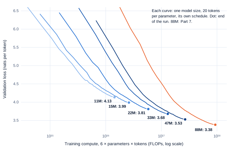
Swipe to pan the diagram, or tap it to zoom.
Early on, bigger models sit higher. Partly that’s size, but it’s also batch: with 4 to 8 times more tokens per step, the 47M and 88M runs take fewer, bigger steps through their first few hundred million tokens.
Predicted against measured hours
The plan, made from short pilot runs, predicted 11.0 hours of training steps for all seven runs. They took 11.76, and every run was 4 to 7% slower than planned:
| Run | Planned tokens/s | Measured tokens/s | Planned hours | Hours of steps | Whole job, hours |
|---|---|---|---|---|---|
| 11M | 178,000 | 165,888 | 0.34 | 0.37 | 0.38 |
| 15M | 125,000 | 117,268 | 0.66 | 0.70 | 0.72 |
| 22M | 105,000 | 99,981 | 1.17 | 1.22 | 1.26 |
| 33M | 70,000 | 65,779 | 2.61 | 2.78 | 2.83 |
| 47M | 51,500 | 47,911 | 5.09 | 5.47 | 5.53 |
| 11M, IsoFLOP | 178,000 | 165,319 | 0.62 | 0.67 | 0.69 |
| 22M, IsoFLOP | 105,000 | 100,609 | 0.52 | 0.55 | 0.57 |
Most of the gap came from the statistic the plan used, the median step’s speed. About every 34 seconds, a step of the small models took about 2 seconds longer. In those same seconds the nvidia-smi logger, a separate process, also skipped samples, so the stall sits below PyTorch, in WSL or the driver; its cause wasn’t traced. The stalls cost the 11M and 22M runs 5 to 6% of their time and barely move the median. The 11M pilot already showed it, at a median of 177,778 tokens per second and a mean of 165,584; the full run’s mean was 165,982.
The 47M model’s pilot had the same gap between median and mean, 5%. The other 2% went to clocks: for about 1.5 hours mid-run the power limit sagged to about 46.6 W and the SM clock to 1,800 MHz. Planned from the pilot’s total tokens over total time, the 11M run would have come within 0.3%.
Part 5’s 22M model, revisited
Part 5’s 22M model reached 4.97 on 230.7 million tokens; this sweep’s 22M model reached 3.81 on 440.5 million. Two things changed: the tokens nearly doubled, and the batch fell from 524,288 tokens per step to 131,072. The IsoFLOP run separates them. It’s the same model with the sweep’s batch, on 197.5 million tokens, fewer than Part 5 used, and it finished at 4.08 on the whole validation shard against Part 5’s 4.97.
| 22M run | Tokens | Tokens per step × steps | Whole-shard loss |
|---|---|---|---|
| Part 5 | 230.7M | 524,288 × 440 | 4.97 |
| Sweep, IsoFLOP | 197.5M | 131,072 × 1,507 | 4.08 |
| Sweep, main | 440.5M | 131,072 × 3,361 | 3.80 |
So about 0.89 of the 1.17 gap came from taking 3.4 times more steps on fewer tokens, and 0.29 from more than doubling the tokens. Part 5 had warned that its 524,288-token batch wasted tokens early in a short run; at 10.5 tokens per parameter the whole run was early.
Step 3: fitting the power law
Losses on the whole validation shard
train.py checks a fixed 4% sample of the validation shard. The fit uses the whole 15-million-token shard, measured once per final snapshot with Part 7’s snapshots.py. Run from the folder that holds runs/, with the shared code on the path:
from snapshots import load, val_loss
from sizes import S47

model = load("runs/s47/model_03601.pt", cfg=S47)   # the final weights-only snapshot
print(val_loss(model))                               # (loss, tokens) over the whole val shard
(3.5134689807891846, 14991360)| Model | Subset (655,360 tokens) | Whole shard (14,991,360 tokens) |
|---|---|---|
| 11M | 4.1346 | 4.1201 |
| 15M | 3.9890 | 3.9731 |
| 22M | 3.8115 | 3.7973 |
| 33M | 3.6807 | 3.6638 |
| 47M | 3.5284 | 3.5135 |
| 88M (Part 7) | 3.3823 | 3.3651 |
The subset is 0.014 to 0.017 harder than the whole shard for every size. To see how much a single run can wobble, the 11M model trained a second time with seed 1338, which changes only the initial weights. It finished at 4.1289 on the whole shard, 0.0088 above the first. One repeat is a rough gauge, but it says differences of a hundredth or so are within noise.
Two forms of the law
A power law says loss is a constant times the parameter count raised to a fixed negative power: L = K × N^-a. On log-log axes that’s a straight line (Math Part 15 fits one by least squares). Chinchilla’s form adds a floor: L = E + A × N^-α, where E is the loss no model size can beat, roughly the randomness left in text, and only the part above it shrinks as a power law. The fit below grids over the exponent; for each value, E and A come from ordinary least squares:
import numpy as np

# final loss on the whole validation shard; total and non-embedding parameters
L     = np.array([4.1201, 3.9731, 3.7973, 3.6638, 3.5135, 3.3651])
N_tot = np.array([10.94, 14.75, 22.03, 32.94, 47.20, 88.10]) * 1e6
N_ne  = np.array([3.07, 5.31, 9.44, 17.21, 28.32, 62.93]) * 1e6

def power_law(N, L):                      # L = K * N^-a, a straight line in logs
    slope, logK = np.polyfit(np.log(N), np.log(L), 1)
    return -slope, np.exp(logK)

def with_floor(N, L):                     # L = E + A * N^-alpha
    best = None
    for alpha in np.arange(0.02, 2.0, 0.0005):        # for each alpha, E and A are linear
        X = np.stack([np.ones_like(N), N ** -alpha], 1)
        (E, A), *_ = np.linalg.lstsq(X, L, rcond=None)
        sse = ((X @ [E, A] - L) ** 2).sum()
        if A > 0 and (best is None or sse < best[0]):
            best = (sse, alpha, E, A)
    return best[1:]

for name, N in (("total", N_tot), ("non-embedding", N_ne)):
    a, K = power_law(N, L)
    alpha, E, A = with_floor(N, L)
    print(f"{name:13}  power law a = {a:.3f}   with floor: alpha = {alpha:.3f}, E = {E:.2f}")
    a5, K5 = power_law(N[:5], L[:5])
    al5, E5, A5 = with_floor(N[:5], L[:5])
    print(f"{'':13}  88M from the five: {K5 * N[5] ** -a5:.3f} (power law), "
          f"{E5 + A5 * N[5] ** -al5:.3f} (with floor), measured {L[5]}")
total power law a = 0.098 with floor: alpha = 0.365, E = 2.69
88M from the five: 3.287 (power law), 3.323 (with floor), measured 3.3651
non-embedding power law a = 0.068 with floor: alpha = 0.134, E = 1.82
88M from the five: 3.327 (power law), 3.313 (with floor), measured 3.3651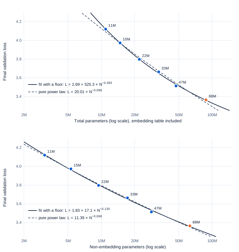
Swipe to pan the diagram, or tap it to zoom.
Against total parameters the points bend: the straight line misses by up to 0.03, and the fit with a floor cuts the typical miss from 0.024 to 0.010. Against non-embedding parameters they nearly line up, and the floor adds almost nothing (0.014 to 0.011). Kaplan et al. saw the same thing across depths: “When we exclude embedding parameters, the performance of models with different depths converge to a single trend.” Here the embedding table is a shrinking share of each larger model, and removing it straightens the curve.
How much to trust six points
A fit with three free constants through six points has three points to spare, and the uncertainty shows. Two checks: leave each point out in turn and refit, and a residual bootstrap, which adds the fit’s own misses back in random order and refits 1,000 times.
| Fit | Exponent | Leave one out | Bootstrap 95% | Floor E (leave one out) |
|---|---|---|---|---|
| Power law, total N | 0.098 | 0.094 to 0.107 | not run | no floor |
| Power law, non-embedding N | 0.068 | 0.067 to 0.071 | not run | no floor |
| With floor, total N | 0.365 | 0.24 to 0.42 | 0.23 to 0.50 | 2.69 (2.10 to 2.81) |
| With floor, non-embedding N | 0.135 | 0.03 to 0.19 | 0.03 to 0.24 | 1.83 (−4.15 to 2.34) |
The power-law exponents are stable. The floor isn’t: on non-embedding counts it moves from −4.15 to 2.34 depending on which point is left out, and a negative floor is meaningless. A floor sits below every measured loss, so pinning it down takes much larger models. The fit’s typical miss, 0.010, is about the seed repeat’s 0.0088: the curve fits as well as the noise allows.
Forecasting the 88M model
Fitted on the five sweep models alone, the four laws put the 88M model between 3.287 and 3.327. It measured 3.365, 0.04 to 0.08 worse: 1 to 2% of the loss, but four to nine times the seed gap. Three explanations fit, and these runs can’t separate them. The curve may bend more than any of these forms allows. The 88M run used a peak rate 0.77 times the sweep’s rule, and 524,288-token steps chosen before this sweep existed. And it’s one seed. The forecast reached nearly twice the size of the largest model in the fit and still landed within 2%.
Step 4: against Kaplan and Chinchilla
Comparing shapes, not levels
Fundamentals Part 12 tells how Kaplan’s and Chinchilla’s laws came about. They were fitted on other text with other tokenizers, so their losses can’t be compared with ours; a nat per token means a different amount of text in each setup. Their exponents and shapes can. Evaluated at our six sizes, along 20 tokens per parameter:
| Law | Its form, as published | Exponent at our sizes | Ours |
|---|---|---|---|
| Kaplan et al. (2020), eq. 1.1 | L(N) = (Nc/N)^αN, non-embedding N, αN ≈ 0.076 | 0.076; 0.075 with their Table 2 data term at D = 20N | 0.068 (0.067 to 0.071) |
| Hoffmann et al. (2022), eq. 10 | E + A/N^0.34 + B/D^0.28, E = 1.69, A = 406.4, B = 410.7 | 0.31 for the part above the floor | 0.37 (0.23 to 0.50) |
| Besiroglu et al. (2024), eq. 3 | 1.8172 + 482.01/N^0.3478 + 2085.43/D^0.3658 | 0.36 for the part above the floor | 0.37 (0.23 to 0.50) |
Along D = 20N, Chinchilla’s two penalty terms both shrink as N grows, one with exponent 0.34 and one with 0.28, so their sum falls with an exponent between them: 0.31 for the paper’s constants, 0.36 for the Epoch AI refit. Both sit inside our fit’s interval of 0.23 to 0.50, and Kaplan’s 0.076 is close to our 0.068, with the caveat that Chinchilla’s law is extrapolated here below the 70 million parameters it started at. The floors, 2.69 here against 1.69 or 1.82, can’t be compared: E depends on the data and tokenizer, and ours is the least certain number in the fit.
Why the counting convention matters
The same six losses give an exponent of 0.098 against total parameters and 0.068 against non-embedding ones, because the first count spans an 8-fold range and the second a 20-fold range. Pearce and Song (2024) traced much of the gap between Kaplan’s advice (optimal size growing as compute to the 0.73) and Chinchilla’s (0.50) to exactly this: Kaplan counted “non-embedding rather than total parameters, combined with their analysis being performed at small scale.” Simulating Chinchilla’s study that way gave them coefficients of 0.74 to 0.78. They recommend that “future scaling studies use total parameters and compute,” which is the convention this series uses for its budgets.
Step 5: was 20 tokens per parameter right?
Three runs, one budget
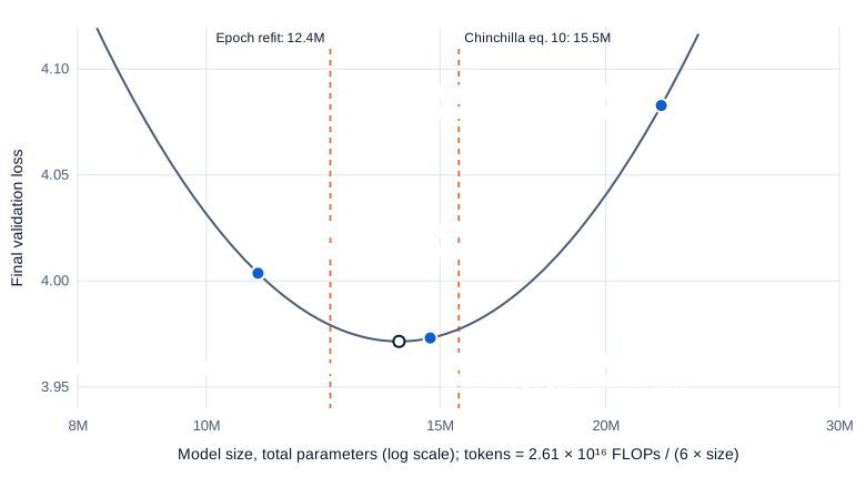
Swipe to pan the diagram, or tap it to zoom.
At equal compute, the 15M model at 20 tokens per parameter beat the 11M model at 36.4 by 0.031 and the 22M model at 9.0 by 0.110. A parabola in the logarithm of size through the three points, the method Llama 3’s paper uses on its own IsoFLOP curves, has its minimum at 14.0 million parameters and 22.3 tokens per parameter. Adding noise the size of the seed repeat to each point and refitting 20,000 times keeps the minimum between 20.8 and 24.8 in 90% of cases. That doesn’t cover the parabola itself, which three points can’t test.
The published laws, extrapolated down to this budget, agree: Chinchilla’s equation 10 puts the optimum at 15.5 million parameters (18 tokens per parameter), the unrounded constants at 17.9 million (13.6), the Epoch refit at 12.4 million (28.2). The curve is lopsided, too. Going to 1.8 times the tokens cost 0.031; going to 2.2 times fewer cost 0.110. Training too briefly hurts more than training a smaller model too long.
What it says about the 88M model
The test ran at 2.61 × 10¹⁶ FLOPs, 36 times less than the 88M run’s 9.31 × 10¹⁷. One budget can’t show whether the best ratio drifts with compute, so the answer for 88M is indirect. At the 88M budget, the three published fits put the optimum at 78 million parameters and 25.5 tokens per parameter (paper’s rounded constants), 91.5 million and 18.5 (unrounded), and 77.6 million and 25.7 (Epoch refit). All three sit within 15% of 88 million. And if the bottom of the curve is as flat there as it is here, a ratio off by a third costs around a hundredth of a nat.
So 20 tokens per parameter was a sound call for the 88M model: measured directly at a small budget, and consistent with every published fit at the real one. Counted in non-embedding parameters, the same 15M optimum is 55.5 tokens per parameter; “20” is a rule about total parameters.
In the real world
- Chinchilla’s IsoFLOP study used “a fixed set of 9 different training FLOP counts (ranging from 6 × 10¹⁸ to 3 × 10²¹ FLOPs)” and model sizes up to 16 billion, with “the cosine schedule length to match the number of tokens,” as every run here did. (Hoffmann et al., 2022)
- Llama 3 ran IsoFLOP sweeps “between 6 × 10¹⁸ FLOPs and 10²² FLOPs,” on models from 40M to 16B parameters, fitted “a second-degree polynomial” to each and extrapolated to “a 402B parameter model on 16.55T tokens.” Its IsoFLOP curves “become flatter around the minimum as the compute budget increases,” so Meta trained 405B.
- Besiroglu et al. (2024) at Epoch AI rebuilt Chinchilla’s data from its plots and found the paper’s rounded fit implies “approximately 70 tokens per parameter,” while their refit gives “around 20 tokens per parameter,” in line with the paper’s other two methods.
- DeepSeek LLM fitted batch size and learning rate to compute instead of fixing them: optimal batch grows as compute to the 0.3271 and optimal rate falls as compute to the −0.1250, and near-optimal settings “fall within a broad band range.” Over this sweep’s 19-fold range in compute, those exponents would grow the batch 2.6 times and cut the rate to 0.69; this sweep’s rules grew the batch 4 times and cut the rate to 0.42.
Common misconceptions
- “A scaling law is one exponent.” The same six losses give 0.098 against total parameters, 0.068 against non-embedding parameters and 0.37 for the part above a fitted floor. An exponent means nothing without its form and its parameter count.
- “Small models show nothing about scaling laws.” Models of 11 to 88 million parameters reproduced Kaplan’s exponent within 0.01, put the best ratio at 22 tokens per parameter, and forecast a model twice the largest of them within 2%. They can’t pin down the floor.
- “The irreducible loss is the most reliable part of the fit.” It’s the least: leaving out one of the six points moved it across a range 0.7 nats wide on total counts and 6.5 nats wide on non-embedding counts. It sits below every measurement.
- “20 tokens per parameter is a law of nature.” It’s the optimum for one way of counting parameters, on certain data, at certain budgets. Counted without the embedding table, the same optimum here is 55.5.
Key takeaways
- Five sizes from 11 to 47 million parameters, each to 20 tokens per parameter with its own schedule, took 12 hours on the laptop GPU; with Part 7’s 88M model their losses fall on one smooth curve, from 4.12 to 3.37.
- Against non-embedding parameters the losses form a straight line with exponent 0.068, near Kaplan’s 0.076. Against total parameters they bend, and a fit with a floor gives an exponent of 0.37, near Chinchilla’s 0.34, with wide error bars.
- At equal compute, 20 tokens per parameter beat 36 and 9, and a parabola puts the best ratio at 22. Published fits put the 88M budget’s optimum within 15% of 88 million parameters, so Part 1’s choice holds up.
- Fitted on the five small models, the law forecast the 88M model’s loss 0.04 to 0.08 too low, within 2%; six points pin down exponents far better than the floor.
- Plan run times with total tokens over total time: periodic 2-second stalls made the small models’ median step 6 to 8% faster than their mean, and every run took 4 to 7% longer than planned.
What’s next
A loss of 3.37 nats per token says the 88M model is better than the 47M one, but not how good it is. Part 9 evaluates the base model: perplexity, bits per byte, which can be compared across tokenizers, and few-shot multiple-choice benchmarks, to see what these losses buy in answers.
Further reading
- Scaling Laws for Neural Language Models (Kaplan et al., 2020): the power laws in non-embedding parameters, data and compute, and Figures 5 and 6 on shape and embeddings.
- Training Compute-Optimal Large Language Models (Hoffmann et al., 2022): Chinchilla’s three methods, IsoFLOP profiles and the fitted law with a floor.
- Chinchilla Scaling: A replication attempt (Besiroglu et al., 2024): Epoch AI’s refit of the parametric law and why the original’s intervals were too narrow.
- Reconciling Kaplan and Chinchilla Scaling Laws (Pearce and Song, 2024): how counting non-embedding parameters at small scale shifts the optimal-size exponent.
- The Llama 3 Herd of Models (Llama Team, 2024): Section 3.2.1, IsoFLOP parabolas from 6 × 10¹⁸ to 10²² FLOPs and the extrapolation to 405B.
- DeepSeek LLM: Scaling Open-Source Language Models with Longtermism (Bi et al., 2024): Section 3.1, scaling laws for batch size and learning rate.
- Tensor Programs V: Tuning Large Neural Networks via Zero-Shot Hyperparameter Transfer (Yang et al., 2022): μP, and why learning rates for Adam’s hidden layers scale with 1/width.