
Beyond Text: Images, Speech and Video · Part 1 of 13
How AI Sees, Hears and Draws: Everything Becomes Tokens
Images, audio and video all become sequences of vectors before a transformer sees them: a measured token ledger across eight open models and Claude.
On this page
TL;DR
Every model in this series, whether it reads a photo, transcribes a meeting or paints a picture, first turns its input into a sequence of vectors. Some of those are discrete tokens, integer IDs from a fixed codebook, like text tokens. Others are continuous latents, grids of real numbers that a network learned to compress the signal into. This article measures that conversion for a self-made picture, synthetic sound and synthetic video, across eight open models and Claude’s API: how many positions and numbers each produces, and how much smaller that is than the raw input. It also maps the other twelve parts of the series onto the two halves of the field, understanding and generation.
Why it matters
The same 512 × 512 picture costs 361 visual tokens on Claude, 324 tokens on Qwen2-VL and 1,088 on SmolVLM. Stable Diffusion’s autoencoder squeezes it into 16,384 numbers, 48 times fewer than its pixels, and a VQ-GAN into 1,024 integers, 473 times fewer bits. Whisper turns one second of audio into 1,500 vectors, the same number it produces for thirty seconds.
Those numbers decide what a model costs to run, how much of the context window an input fills, and what detail survives. Shown 6 to 17 small red dots at 150 × 100 pixels, 27 image tokens, Claude Haiku 5.5 counted them exactly in 10 of 40 scenes; at 1200 × 800 it got all 40 right.
Fundamentals Part 15 explained the main designs: patches, CLIP, projectors, Whisper and codec tokens. This part measures them on a laptop GPU and maps the rest of the series.
The intuition
Think of a shipping port. Cargo arrives as anything: grain, cars, furniture. Before a crane can lift it, it’s packed into standard containers. The crane is the transformer from Fundamentals Part 6, and it only lifts containers: fixed-length vectors, one per sequence position.
Each modality has its own packing station. An image is cut into tiles. Sound is sliced into short time steps. Some stations write a catalog number on each container instead of packing the goods themselves; that’s a discrete token, and someone at the far end must keep the catalog to unpack it.
The analogy breaks at the packing itself. A port leaves the cargo as it is, while these packers learn what to keep. A good image autoencoder throws away pixel noise you’d never notice and keeps edges and color. A bad one, or one pushed too hard, throws away the text on a sign. How much gets lost is a design choice made when the packer is trained.
Two halves: understanding and generation
The field splits along the direction the vectors flow.
Understanding runs encoders forward: pixels or sound in, vectors out, and a language model reads them next to your text. The vectors only need to be useful to the reader, so they can be continuous, and they rarely need to be turned back into pixels.
Generation has to come back out. A model that draws or speaks produces a sequence, then a decoder turns it into pixels or a waveform. Two families do this. Diffusion models start from noise in a continuous latent space and remove it step by step. Autoregressive models predict discrete tokens one at a time, as a language model predicts words, and a codec decoder turns the tokens back into an image or sound.

Swipe to pan the diagram, or tap it to zoom.
The series follows that split:
- Part 2, vision transformers: how a ViT turns patches into vectors, and why its cost grows with the square of resolution.
- Part 3, CLIP and contrastive learning: how images and captions are trained into one shared space.
- Part 4, vision-language models: the connectors that feed image vectors into a language model, and what image tokens cost.
- Part 5, diffusion from scratch: the denoising math, with a tiny model trained on the laptop.
- Part 6, latent diffusion: the autoencoder, the U-Net and guidance in Stable Diffusion, run and timed.
- Part 7, diffusion transformers and flow matching: the design behind the SD3 and FLUX family.
- Part 8, autoregressive and unified image generation: image tokens predicted like text.
- Part 9, speech recognition with Whisper: log-mel spectrograms and word error rate, measured.
- Part 10, text-to-speech: stock voices, neural codecs and real-time factor.
- Part 11, audio tokens and voice agents: codecs, speech-to-speech models and the latency budget.
- Part 12, video generation: spacetime patches and video diffusion.
- Part 13, serving multimodal models: token costs, encoder caching and a review of the series.
Parts 2 to 4 and 9 are about understanding; Parts 5 to 8, 10 and 12 are about generation; Parts 11 and 13 need both.
Step 1: one picture, six representations
The test picture is a scene drawn in code: a sky gradient, a sun, two hills, a house, a tree, a ball and a row of twelve small red dots. No photo, no faces. It’s drawn in relative coordinates, so every size shows the same scene. At 512 × 512 pixels with three color channels it holds 786,432 numbers of 8 bits each.
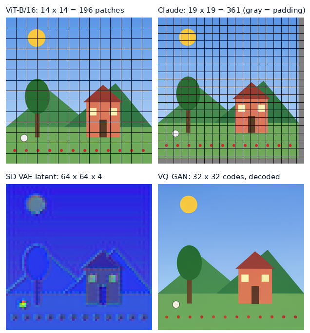
Patches for an encoder
A Vision Transformer (ViT) cuts the image into square patches and turns each into one vector, as Fundamentals Part 15 showed with NumPy. Running the real thing, google/vit-base-patch16-224 (86M parameters, Apache-2.0), on the test picture:
import torch
from PIL import Image
from transformers import ViTImageProcessor, ViTModel

img = Image.open("scene.png").convert("RGB")                    # 512 x 512
proc = ViTImageProcessor.from_pretrained("google/vit-base-patch16-224")
vit = ViTModel.from_pretrained("google/vit-base-patch16-224", dtype=torch.bfloat16, device_map="cuda")
x = proc(images=img, return_tensors="pt")["pixel_values"]       # (1, 3, 224, 224)
with torch.no_grad():
    print(vit(pixel_values=x.to("cuda", torch.bfloat16)).last_hidden_state.shape)
# torch.Size([1, 197, 768])
The processor first shrinks the picture to 224 × 224, so 81% of the pixels are gone before the model sees anything. Then 14 × 14 = 196 patches plus one class token give 197 vectors of 768 numbers: 151,296 numbers in all. That’s 5.2 times fewer than the 512-pixel original but almost exactly as many as the 224-pixel input (150,528). Each 16 × 16 × 3 patch of 768 pixel values becomes 768 learned features, which also carry information from the other patches, so the encoder has re-described the picture at the same size.
Image tokens for a language model
A vision-language model (VLM) feeds such vectors into a language model, and each one takes a position in the context window, the same as a word. The processors of two open VLMs, run on the same picture at three sizes, gave:
| Picture | Qwen2-VL-2B tokens | SmolVLM-256M tokens | Claude (formula) |
|---|---|---|---|
| 224 × 224 | 64 | 1,088 | 64 |
| 512 × 512 | 324 | 1,088 | 361 |
| 1024 × 1024 | 1,369 | 1,088 | 1,369 |
Qwen2-VL’s count follows the image: 14-pixel patches, then each 2 × 2 block merged into one token, so 512 pixels (rounded to 504) gives 36 × 36 / 4 = 324. SmolVLM’s processor does something else: it scales every image so the long edge is 2,048 pixels, cuts that into 4 × 4 tiles of 512 plus one shrunk copy of the whole image, and compresses each tile to 64 tokens. A 224-pixel thumbnail is blown up nine times along each side and costs 1,088 tokens, 17 times what Qwen2-VL charges for it. That’s a default in preprocessor_config.json, not a fact about images. Part 4 measures what those tokens buy.
Claude’s image tokens, counted
Anthropic’s vision docs give the rule: one visual token per 28 × 28-pixel patch, ⌈width / 28⌉ × ⌈height / 28⌉. Models from Claude 4.7 on, which includes Haiku 5.5, accept up to 2,576 pixels on the long edge and 4,784 visual tokens; larger images are shrunk, keeping their shape, to the biggest size that fits both limits.
The free token-counting endpoint shows what a request will cost without running it. Sending the same picture at ten sizes to claude-haiku-5-5, and subtracting the count for the text-only request (35 tokens):
| Picture sent | Shrunk by the API to | Formula | Measured image tokens |
|---|---|---|---|
| 150 × 100 | not shrunk | 6 × 4 = 24 | 27 |
| 300 × 200 | not shrunk | 11 × 8 = 88 | 91 |
| 600 × 400 | not shrunk | 22 × 15 = 330 | 333 |
| 900 × 600 | not shrunk | 33 × 22 = 726 | 729 |
| 1200 × 800 | not shrunk | 43 × 29 = 1,247 | 1,250 |
| 1800 × 1200 | not shrunk | 65 × 43 = 2,795 | 2,798 |
| 2400 × 1600 | 2352 × 1568 | 84 × 56 = 4,704 | 4,707 |
| 3000 × 2000 | 2352 × 1568 | 84 × 56 = 4,704 | 4,707 |
| 4000 × 500 | 2576 × 322 | 92 × 12 = 1,104 | 1,107 |
| 500 × 4000 | 322 × 2576 | 12 × 92 = 1,104 | 1,107 |
Every one is the formula plus 3, the overhead Agentic AI Part 9 found for screenshots, and the docs’ reference resize function predicted every shrunk size.
Real calls are billed the same way. Three Haiku 5.5 calls (thinking disabled, a one-line question, at most 16 output tokens) at 300 × 200, 1200 × 800 and 3000 × 2000 reported usage.input_tokens of 124, 1,283 and 4,740: in each case exactly 2 fewer than the counting endpoint’s total for the same request, so the endpoint’s count runs 2 tokens high for the whole request, not per image. The three calls cost $0.00062 together. At Haiku 5.5’s $0.10 per million input tokens, a 1200 × 800 picture costs $0.13 per thousand images and anything at the cap $0.48 per thousand, half that through the Batch API.
The token count also limits what detail reaches the model. The same scene with 6 to 17 red dots (40 scenes, dot counts drawn with a fixed seed), each sent at five sizes to Haiku 5.5 with thinking disabled, 200 requests through the Batch API, asked for the number of dots:
| Size sent | Image tokens | Exact count (95% CI) | Mean miss |
|---|---|---|---|
| 150 × 100 | 27 | 10 of 40, 25% (14-40) | 1.65 dots |
| 300 × 200 | 91 | 16 of 40, 40% (26-55) | 0.70 dots |
| 600 × 400 | 333 | 29 of 40, 73% (57-84) | 0.28 dots |
| 1200 × 800 | 1,250 | 40 of 40, 100% (91-100) | 0 |
| 2400 × 1600 | 4,707 | 36 of 40, 90% (77-96) | 0.10 dots |
The intervals are Wilson intervals, as in Measuring LLMs Part 3. At 150 × 100 a dot is 3 pixels wide and several dots share one 28-pixel patch; the model undercounted, by 5 or 6 on the 17-dot scenes. At 600 × 400 all 11 misses were one too many. Beyond 1,250 tokens nothing improved: the four misses at 2400 × 1600 were 16- and 17-dot scenes counted one short that 1200 × 800 got right, and 4 such pairs against 0 isn’t significant on its own (exact McNemar test, p = 0.125). Every reply was a bare number, none cut off. The whole batch cost $0.013. Part 4 runs tasks like this across several models.
Latents for a generator
A generator needs the reverse trip as well, so its representation must be decodable. Latent diffusion (Rombach et al., 2021) trains an autoencoder first: an encoder that “downsamples the image by a factor f”, and a decoder that rebuilds it. The paper tried f from 1 to 32 and found that f between 4 and 16 “strike a good balance between efficiency and perceptually faithful results”. Stable Diffusion’s variational autoencoder (VAE) uses f = 8 with 4 channels. A VAE is an autoencoder trained so its latents stay close to a smooth, roughly Gaussian distribution, which keeps the latent space well behaved for the diffusion model.
stabilityai/sd-vae-ft-mse (MIT license), run on the test picture in bfloat16:
import numpy as np
from diffusers import AutoencoderKL

vae = AutoencoderKL.from_pretrained("stabilityai/sd-vae-ft-mse", torch_dtype=torch.bfloat16).to("cuda")
x = torch.from_numpy(np.asarray(img)).permute(2, 0, 1)[None].div(127.5).sub(1)   # (1, 3, 512, 512) in [-1, 1]
with torch.no_grad():
    z = vae.encode(x.to("cuda", torch.bfloat16)).latent_dist.mean
print(z.shape)                           # torch.Size([1, 4, 64, 64])
That’s 16,384 numbers, 48 times fewer than the pixels, and the decoder rebuilt the picture at a peak signal-to-noise ratio (PSNR) of 40.2 dB. PSNR compares the rebuilt picture with the original pixel by pixel, on a log scale; above about 30 dB the differences are hard to see. In the figure the latent still looks like the scene, a small blurry map of it, because each of the 64 × 64 cells describes one 8 × 8-pixel block. Part 6 runs the whole pipeline on it.
Discrete codes for a generator
The other route turns the image into integers. VQ-VAE (van den Oord et al., 2017) adds a codebook to the autoencoder: a table of learned vectors, and each latent cell is replaced by the ID of its nearest entry. The paper compressed 128 × 128 × 3 images into a 32 × 32 grid of IDs from a 512-entry codebook, “a reduction of ≈ 42.6 in bits”. Once an image is a grid of IDs, a transformer can predict it one token at a time, like text.
The VQ-GAN inside aMUSEd (Patil et al., 2024; amused/amused-256, OpenRAIL++ license) downsamples by 16 and has 8,192 codebook entries, so each ID carries 13 bits. On the test picture:
| Input | Code grid | Codes | Bits | Reduction in bits | PSNR |
|---|---|---|---|---|---|
| 256 × 256 | 16 × 16 | 256 | 3,328 | 473× | 30.5 dB |
| 512 × 512 | 32 × 32 | 1,024 | 13,312 | 473× | 34.9 dB |
The 512-pixel picture used 391 distinct codes out of 8,192. In the figure every shape survives, but up close the red dots come back duller and slightly misshapen and the white ball turns cream: no codebook entry matches those exact colors, so each cell takes its nearest. About 11 times fewer bits than VQ-VAE’s 2017 setting buys a sequence short enough to generate token by token, and the price is color and fine edges. Part 8 covers models that generate images this way.
Step 2: sound and video
Audio as frames for an encoder
Whisper (Radford et al., 2022) resamples audio to 16,000 Hz and computes, in the paper’s words, “an 80-channel log-magnitude Mel spectrogram representation” on “25-millisecond windows with a stride of 10 milliseconds”: a picture of sound with 100 columns per second, each describing how much energy falls in 80 pitch bands. Two convolutions, the second with stride 2, halve that to 50 encoder positions per second, over a fixed 30-second window.
With openai/whisper-tiny (39M parameters, Apache-2.0) on synthetic tones (a chord and a rising chirp, no voice):
| Clip | Samples | Log-mel features | Encoder output |
|---|---|---|---|
| 1 s | 16,000 | 80 × 3,000 | 1,500 × 384 |
| 10 s | 160,000 | 80 × 3,000 | 1,500 × 384 |
| 30 s | 480,000 | 80 × 3,000 | 1,500 × 384 |
Every clip gives the same shape, because the feature extractor pads it with silence to 30 seconds. The tiny model’s encoder turns one second of audio into 1,500 vectors of 384 numbers, 576,000 numbers for 16,000 samples: 36 times more than it started with. Per second of a full window, that’s 50 positions and 19,200 numbers, still more than the raw audio. Whisper’s encoder exists to transcribe, and Part 9 measures how well it does that in word error rate.
Audio as codec tokens
A neural audio codec turns sound into integer codes and back, the audio counterpart of VQ-GAN. EnCodec (Défossez et al., 2022) produces “75 latent steps per second of audio at 24 kHz” and quantizes each with residual vector quantization (RVQ): a stack of codebooks of 1,024 entries, each one coding what the previous ones missed. Keeping 2, 4, 8, 16 or 32 codebooks gives 1.5 to 24 kbps, so 150 to 2,400 tokens per second.
Kyutai’s Mimi codec, from the Moshi paper, runs at only 12.5 frames per second. Its weights, kyutai/mimi (CC-BY-4.0), on ten seconds of the same tones at 24 kHz:
| Codebooks kept | Code grid for 10 s | Tokens per second | Bitrate | Signal-to-noise of the rebuilt audio |
|---|---|---|---|---|
| 8 (Moshi’s setting) | 8 × 125 | 100 | 1.1 kbps | 3.7 dB |
| 32 (all) | 32 × 125 | 400 | 4.4 kbps | 7.0 dB |
Each code is one of 2,048 entries, 11 bits. Raw 16-bit audio at 24 kHz is 384 kbps, so 8 codebooks are 349 times smaller. The low signal-to-noise figures are expected. The Moshi paper trained Mimi with adversarial losses only, dropping the reconstruction losses, and reports that this “majorly degrades objective metrics” while listeners rated the audio better. A waveform comparison on a synthetic chord therefore says how far the codes drift from the exact samples, not how good they sound. Even 100 tokens per second is a lot: the Moshi paper notes English speech is about “3 to 4 text tokens per second”, so a voice model’s sequence is about 30 times longer than the transcript’s. Parts 10 and 11 work with these codes.
Video: frames times patches, or spacetime patches
A video is a stack of frames, and the simplest way in multiplies everything: frames per second times patches per frame. At 24 frames per second, ViT-B/16 would produce 24 × 197 = 4,728 vectors for every second, and Stable Diffusion’s VAE 24 × 16,384 = 393,216 numbers.
Models cut this two ways. They sample fewer frames, and they fold neighboring frames together. ViViT (Arnab et al., 2021) introduced tubelet embedding: it cuts the video into non-overlapping tubes through space and time, so one token covers a 16 × 16-pixel square across 2 frames. Building ViViT-B/16x2’s embedding layer from its published configuration (random weights, shapes only) and feeding it a 32-frame 224 × 224 clip gives 3,137 vectors: 16 time steps × 14 × 14 patches, plus one class token, half what per-frame patches would give.
Qwen2-VL does both: it samples 2 frames per second and folds each pair into one set of patches. Its processor turned 4 seconds of synthetic video at 448 × 448 (8 frames) into a grid of 4 × 32 × 32 patches and 1,024 tokens, which is 256 tokens per second. Part 12 covers spacetime patches for video generation, where the same idea runs on a compressed latent video instead of pixels.
Step 3: the token ledger
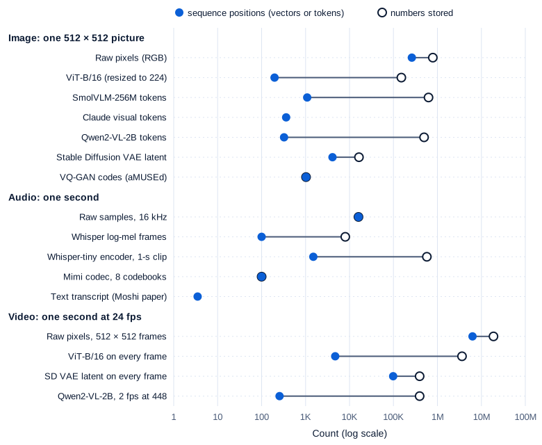
Swipe to pan the diagram, or tap it to zoom.
The same numbers as a table, with the reduction from raw input:
| Input | Representation | Positions | Numbers | Reduction from raw |
|---|---|---|---|---|
| Picture | Raw RGB pixels, 512 × 512 | 262,144 | 786,432 | 1× |
| Picture | ViT-B/16 vectors (resized to 224) | 197 | 151,296 | 5.2× |
| Picture | Qwen2-VL-2B tokens, width 1,536 | 324 | 497,664 | 1.6× |
| Picture | Stable Diffusion VAE latent | 4,096 | 16,384 | 48× |
| Picture | VQ-GAN codes, 13 bits each | 1,024 | 1,024 | 473× in bits |
| Audio, 1 s | Raw samples, 16 kHz | 16,000 | 16,000 | 1× |
| Audio, 1 s | Whisper log-mel frames | 100 | 8,000 | 2× |
| Audio, 1 s | Whisper-tiny encoder (padded clip) | 1,500 | 576,000 | 36× larger |
| Audio, 1 s | Mimi codes, 8 codebooks of 11 bits | 100 | 100 | 349× in bits (from 24 kHz) |
| Video, 1 s at 24 fps | Raw 512 × 512 frames | 6.3M | 18.9M | 1× |
| Video, 1 s at 24 fps | ViT-B/16 on every frame | 4,728 | 3.6M | 5.2× |
| Video, 1 s at 24 fps | SD VAE latent on every frame | 98,304 | 393,216 | 48× |
| Video, 1 s at 24 fps | Qwen2-VL-2B, 2 fps at 448 | 256 | 393,216 | 48× |
The representations built for understanding cut positions by a factor of hundreds or more but keep about as many numbers, or add some: they exist to be read, and attention’s cost grows with the square of the positions (a raw-pixel sequence of 262,144 would need an attention map 1.8 million times larger than ViT’s 197). The representations built for generation cut the numbers too, by 48 to 473 times, because a generator must produce every one of them.
How long the packing takes, on the laptop’s NVIDIA GeForce RTX 4060 Laptop GPU (8 GB) in bfloat16, PyTorch 2.11 and driver 592.82, median of at least 5 timed runs after 3 warm-ups with torch.cuda.synchronize() around each, and the clock and power read with nvidia-smi during the runs:
| Step | Median time | Timed runs | SM clock | Power |
|---|---|---|---|---|
| ViT-B/16, one 224-pixel image | 9.2 ms (4.8-23.9) | 97 | 1,635 MHz | 19 W |
| ViT-B/16, 24 frames in one batch | 48.7 ms | 21 | 1,748 MHz | 42 W |
| SD VAE encoder, one 512-pixel image | 87.1 ms | 12 | 1,943 MHz | 43 W |
| SD VAE encoder, 8 frames in one batch | 713 ms | 5 | 1,980 MHz | 44 W |
| VQ-GAN encode and quantize, 512 pixels | 70.8 ms | 15 | 2,085 MHz | 47 W |
| Whisper-tiny encoder, one 30-s window | 2.8 ms | 200 | 2,100 MHz | 45 W |
| Mimi encoder, 10 s, 8 codebooks | 28.0 ms | 36 | 2,100 MHz | 33 W |
The single ViT image is too small to keep the GPU busy, which is why its clock and power stay low and its times spread so widely. The VAE is the slow packer: at 89 ms a frame, one second of 24-frame video takes about 2.1 seconds to encode frame by frame. Mimi encodes ten seconds of sound in 28 ms, 357 times faster than real time, so encoding is a small part of a voice agent’s latency budget.
In the real world
- Stable Diffusion’s denoiser never sees a pixel, only the 64 × 64 × 4 grid measured above. Diffusion transformers go one step further: DiT (Peebles and Xie, 2022) “patchifies” the latent, so a 256 × 256 image, whose latent is 32 × 32 × 4, becomes 256 tokens with 2 × 2 patches. Stable Diffusion 3 (Esser et al., 2024) widened the latent to 16 channels, finding that “increasing the number of latent channels d significantly boosts reconstruction performance”. Both reported, not reproduced here; Part 7 covers them.
- Voice models fight the codec’s sequence length. The Moshi paper notes that 8 codebooks at 12.5 Hz mean “100 steps per second of audio”, and that “to model 5 minutes of audio, this would amount to 30,000 timesteps”. Moshi’s answer is two transformers: a large one that steps through time at 12.5 Hz and a small one that predicts the 8 codebooks within each step.
- Vision-language models disagree by an order of magnitude on what one picture costs. Claude, Qwen2-VL and SmolVLM gave 64, 64 and 1,088 tokens for the same 224-pixel thumbnail, because each processor resizes and tiles differently. The SmolVLM paper (Marafioti et al., 2025) describes the pixel shuffle that squeezes each 512-pixel tile to 64 tokens.
- Models that put image codes straight into a language model’s vocabulary, like Chameleon in Fundamentals Part 15, inherit both sides of the VQ trade measured above: a short sequence, and colors and edges the codebook can’t quite hit.
Common misconceptions
- “An encoder compresses the image or sound.” Encoders for understanding mostly re-describe. ViT-B/16 turns 150,528 input numbers into 151,296, and Whisper-tiny turns one second of audio into 36 times more numbers than it had samples. Compression is what generators need, because they must model every number they produce.
- “The token count is a property of the image.” It’s a property of the processor. The same 224-pixel picture was 64 tokens for Claude and Qwen2-VL and 1,088 for SmolVLM at its default settings.
- “More image tokens always means better answers.” Counting dots went from 25% exact at 27 tokens to 100% at 1,250, then 90% at 4,707. Past the point where the detail fits in the patches, extra tokens cost money and bought nothing measurable here.
- “A short audio clip is cheap for Whisper.” The feature extractor pads every clip to 30 seconds, so one second of speech goes through the same 1,500 encoder positions as thirty.
- “Discrete tokens are a text thing.” Images and sound become integer IDs too, from a codebook: 1,024 per 512-pixel image for the VQ-GAN here, 100 per second for Mimi. That’s what lets one autoregressive model generate text, images and audio with the same next-token loss.
Key takeaways
- Every modality reaches a transformer as a sequence of vectors: continuous patch vectors, latents or encoder frames, or discrete IDs from a learned codebook.
- Understanding needs vectors a model can read. Generation needs vectors a decoder can turn back into pixels or sound, so it compresses hard: 48 times fewer numbers for Stable Diffusion’s latent, 473 times fewer bits for VQ-GAN codes, 349 times for Mimi.
- Claude’s image cost is one token per 28 × 28-pixel patch plus 3, capped at 4,784 tokens on Haiku 5.5; the counting endpoint measured exactly that at ten sizes, and real calls billed 2 tokens fewer than it counted.
- Tokens decide what survives: Haiku 5.5 counted small dots right 25% of the time at 27 image tokens and every time at 1,250.
- Check the processor before you trust a token count. Resizing, tiling and padding to 30 seconds change the bill more than the content does.
What’s next
Part 2 opens the first packing station properly: the Vision Transformer. It measures what patch size and resolution cost in time and GPU memory against a convolutional network, what happens when you feed a ViT a resolution it never saw in training, and why a transformer with no built-in idea of “nearby pixels” needed hundreds of millions of images to beat one that has it.
Further reading
- High-Resolution Image Synthesis with Latent Diffusion Models (Rombach et al., 2021): the autoencoder’s downsampling factor f and why 4 to 16 works.
- Neural Discrete Representation Learning (van den Oord et al., 2017): VQ-VAE, the codebook idea behind discrete image and audio tokens.
- aMUSEd: An Open MUSE Reproduction (Patil et al., 2024): the open VQ-GAN used here, 16 times downsampling and 8,192 codes.
- Robust Speech Recognition via Large-Scale Weak Supervision (Radford et al., 2022): Whisper’s log-mel input and 30-second window.
- High Fidelity Neural Audio Compression (Défossez et al., 2022): EnCodec, 75 frames per second and bitrate by codebook count.
- Moshi: a speech-text foundation model for real-time dialogue (Défossez et al., 2024): the Mimi codec and the RQ-Transformer that keeps its sequence manageable.
- ViViT: A Video Vision Transformer (Arnab et al., 2021): uniform frame sampling versus tubelet embedding.
- An Image is Worth 16x16 Words (Dosovitskiy et al., 2020): the Vision Transformer and its patch embedding.
- Qwen2-VL (Wang et al., 2024) and SmolVLM (Marafioti et al., 2025): two ways to turn images and video into language-model tokens.
- Scalable Diffusion Models with Transformers (Peebles and Xie, 2022) and Scaling Rectified Flow Transformers (Esser et al., 2024): latents as transformer tokens, and wider latents.
- Vision (Claude API docs) and Coordinates and bounding boxes (Claude API docs): the visual-token formula, resolution tiers and the reference resize function.
- Multimodal Models: How LLMs See and Hear (Fundamentals Part 15): the overview of patches, CLIP, connectors and audio that this series builds on.