
Beyond Text: Images, Speech and Video · Part 6 of 13
Latent Diffusion: How Stable Diffusion Turns Text into Pictures
Stable Diffusion 1.5 taken apart and timed on a laptop GPU: the VAE, the U-Net, CLIP text, classifier-free guidance, negative prompts and samplers, measured.
On this page
TL;DR
Stable Diffusion runs the denoising process of Part 5 on a small compressed grid, a latent, instead of on pixels. A CLIP text encoder reads the prompt, a U-Net removes noise from the latent while looking at the text, and the decoder of a variational autoencoder turns the result into a picture. This article takes Stable Diffusion 1.5 apart on a laptop GPU and measures what an image costs, what the guidance scale does to faithfulness and variety, what a negative prompt really is, and why 20 sampling steps are enough.
Why it matters
A 512 × 512 picture from Stable Diffusion 1.5 took 2.77 seconds on a laptop GPU, and 93% of that time went to one network, the U-Net, run 40 times. Run that U-Net on the pixels instead of on its 64 × 64 latent and each pass would cost 545 trillion arithmetic operations instead of 0.8 trillion: 679 times as many.
One setting decides whether the picture follows the prompt. At a guidance scale of 1, Claude Haiku 5.5 judged 13% of 70 images to show everything their prompt asked for; at 7.5, the usual default, 66%. Past that, faithfulness stopped improving, but the images kept changing: colours grew more saturated and the pictures from different random seeds grew more alike.
Where does the time go, and why does one knob trade faithfulness for variety?
The intuition
Think of an architect and a builder. The architect revises a small floor plan, where moving a wall is cheap; the builder turns the finished plan into a full-size house. Stable Diffusion’s U-Net is the architect, doing 20 or 50 rounds of revision on a 64 × 64 plan. The autoencoder’s decoder is the builder, called once at the end.
Guidance is a second trick. Two copies of the architect look at the same plan, one who has read the client’s brief and one who hasn’t. The difference between their suggestions is what the brief asks for, so you exaggerate it.
The analogy breaks in two places. The plan isn’t a drawing a person could read; it’s four channels of learned numbers. And the decoder doesn’t follow a specification: it invents texture and small detail the plan never stored.
Step 1: why diffuse in a latent
Fundamentals Part 15 sketched image generation in a few lines; this part opens one generator up. A diffusion model, as Part 5 builds it, learns to predict the noise in a noisy image and generates by removing a little noise at a time, each step a full pass through a large network over every number in the image. The latent diffusion paper (Rombach et al., 2021) starts from an observation about what such models spend their effort on: “Most bits of a digital image correspond to imperceptible details.” It splits learning into two stages. A perceptual compression stage, an autoencoder, “removes high-frequency details but still learns little semantic variation”; the diffusion model then does the semantic compression, learning what goes where, in the autoencoder’s smaller space.
Part 1 measured Stable Diffusion’s autoencoder on a 512 × 512 test picture: a latent of 4 × 64 × 64 = 16,384 numbers, 48 times fewer than the 786,432 pixel values, rebuilt at a peak signal-to-noise ratio of 40.2 dB, and 87 ms to encode. Diffusion runs entirely on that grid, after the latent is multiplied by 0.18215, the VAE’s scaling factor, so that it has roughly unit variance like the noise it will be mixed with (the paper’s recipe estimates this from a batch of data).
The cost argument, counted
PyTorch’s FLOP counter can run the U-Net on “meta” tensors, which carry shapes but no data, so it counts the arithmetic for a grid of any size without the memory. A FLOP is one floating-point operation; a multiply-add counts as two.
| Grid the U-Net denoises | What it corresponds to | GFLOP per U-Net pass | Share in attention matrices |
|---|---|---|---|
| 32 × 32 | latent of a 256-pixel image | 180 | 5% |
| 64 × 64 | latent of a 512-pixel image (SD 1.5) | 803 | 16% |
| 128 × 128 | latent of a 1,024-pixel image | 4,674 | 42% |
| 512 × 512 | the 512-pixel image itself, in pixel space | 545,118 | 92% |
The same network on pixels would cost 679 times as much per step. Convolutions grow with the number of positions, but self-attention compares every position with every other: 4,096 positions at the U-Net’s finest level make 16.8 million pairs per head, 262,144 pixels would make 69 billion. Real pixel-space models are built differently, so 679 is an upper bound, but it shows where the argument comes from. With “the same computational budget” on one A100, the paper found that “pixel-based LDM-1 requires substantially larger train times” than downsampling factors 4 to 16, while factor 32 “limits the overall sample quality” (reported, not reproduced here). Factor 8 with 4 channels became Stable Diffusion.
Step 2: the three networks in Stable Diffusion 1.5
stable-diffusion-v1-5/stable-diffusion-v1-5 is an ungated mirror of the original release under the CreativeML OpenRAIL-M license; its card says it was fine-tuned for 595,000 steps at 512 × 512 on the “laion-aesthetics v2 5+” subset of LAION. Everything here uses its fp16 weights (2.7 GB downloaded) on an NVIDIA GeForce RTX 4060 Laptop GPU (8 GB), with diffusers 0.42.1, PyTorch 2.11 and driver 592.82.

| Part | Parameters | Job |
|---|---|---|
| Text encoder | 123.1M | Turns the prompt into 77 × 768 vectors with the text half of CLIP ViT-L/14; frozen during training |
| U-Net | 859.5M | Predicts the noise in the latent, once or twice per step |
| VAE (encoder 34.2M, decoder 49.5M) | 83.7M | Image to latent and back; only the decoder runs for text-to-image |
| Safety checker | 304.0M | An image encoder from the same CLIP model; flags outputs close to hidden concept embeddings |
The text encoder
The prompt is split into tokens, padded or cut to 77 (anything longer is silently dropped), and passed through the text half of OpenAI’s CLIP ViT-L/14, the contrastive model of Part 3. Stable Diffusion keeps all 77 output vectors, not just the pooled one CLIP uses for matching, so the U-Net can look at individual words. The encoder stays frozen; the diffusion model learned to read CLIP’s vectors. It’s the cheapest part: 13 GFLOP and 11.5 ms for a prompt and an empty prompt together.
The U-Net and cross-attention
A U-Net is a convolutional network shaped like a U: it shrinks the grid from 64 × 64 to 32, 16 and 8 while widening the channels from 320 to 1,280, then grows it back, with skip connections carrying detail across from each level on the way down to its twin on the way up. The noise level reaches every block as a time embedding, a vector computed from the step number. Stable Diffusion’s has 22 residual convolution blocks and 16 transformer blocks. Each transformer block runs self-attention (every grid position looks at every other), cross-attention (every position looks at the 77 text vectors) and a small MLP (multilayer perceptron). In cross-attention the queries come from the image and the keys and values from the text:
Q = W_Q · image features     4,096 × 40 per head at the 64 × 64 level
K = W_K · text vectors          77 × 40 per head
V = W_V · text vectors          77 × 40 per head
out = softmax(Q Kᵀ / √40) · V   each grid cell takes a weighted mix of the 77 word vectors
Here 40 is the width of each of the 8 heads (320 channels / 8). Each of the 4,096 positions scores all 77 tokens, turns the scores into weights that sum to 1, and adds the weighted text vectors to its features. That’s how the word “red” ends up affecting some cells more than others. The cross-attention layers hold 44.0M of the U-Net’s 859.5M parameters.
What one image costs
Each row is the median of 20 timed runs after 5 warm-ups (5 for whole images), with torch.cuda.synchronize() around each and the clock and power read with nvidia-smi during the runs:
| Step | Median time | Peak GPU memory | SM clock | Power |
|---|---|---|---|---|
| Text encoder, prompt + empty prompt | 11.5 ms | 2.78 GB | 1,620 MHz | 11 W |
| U-Net, one pass (batch 1) | 80.2 ms | 2.86 GB | 1,740 MHz | 39 W |
| U-Net, guided step: 2 passes batched | 128.7 ms | 2.91 GB | 1,913 MHz | 43 W |
| U-Net, guided step: 2 passes one after the other | 180.8 ms | 2.86 GB | 2,108 MHz | 42 W |
| VAE decode, 64 × 64 to 512 × 512 | 182.4 ms | 3.42 GB | 1,935 MHz | 46 W |
| Safety checker | 33.8 ms | 2.79 GB | 2,175 MHz | 23 W |
| Whole image: DPM-Solver++, 20 steps, guidance 7.5 | 2.77 s | 3.42 GB | 1,905 MHz | 46 W |
| Whole image: same, guidance off (scale 1) | 1.85 s | 3.42 GB | 1,935 MHz | 45 W |
| Whole image: PNDM (the shipped default), 50 steps | 6.72 s | 3.42 GB | 1,920 MHz | 47 W |
The weights take 2.77 GB, so the pipeline uses less than half the card. Twenty guided steps at 128.7 ms are 2.57 s, 93% of the image. The VAE decoder is the most expensive single call, 2,515 GFLOP or more than three U-Net passes, because its last layers work at full resolution; it runs once, so it’s 7% of the image. The U-Net reached 12.5 TFLOPS (2 × 803 GFLOP in 128.7 ms), about half the 25.3 TFLOPS that GPU Part 4 measured for 16-bit matrix multiplies on this GPU.
diffusers uses PyTorch’s fused scaled dot-product attention (SDPA) by default, which never writes the full attention matrix to memory. The classic implementation, which does, made a guided step 44% slower (185.6 ms) and used 1.0 GB more memory; attention slicing, which computes the heads in chunks to save memory, was slower still (188.0 ms).
What the safety checker does
The diffusers source shows what the final filter is: a CLIP ViT-L/14 image encoder that compares the finished picture, by cosine similarity, with 17 concept embeddings and 3 “special care” ones, each with its own threshold. The concepts are “intentionally hidden to reduce the likelihood of reverse-engineering this filter,” per the model card. If any similarity passes its threshold, the image is replaced by a black one. It runs after generation, in 33.8 ms, and changes nothing the U-Net does.
Of the 704 images generated for the experiments below, all of food, animals, objects and landscapes, it flagged 5 (0.7%, 95% Wilson interval 0.3% to 1.7%): a glowing jellyfish, two stacks of pancakes and two slices of chocolate cake. They’re left out of every score. The other 699 sat a median of 0.046 below their nearest threshold.
Step 3: classifier-free guidance
A model that simply learns “images given captions” follows the caption loosely. Classifier-free guidance (Ho and Salimans, 2022) turns that up with one training trick: replace the caption with an empty one for a fraction of examples, so one network learns both the conditional prediction (with the text) and the unconditional one (without). Stable Diffusion 1.5 was trained with “10% dropping of the text-conditioning,” per its card; the paper found 10% and 20% worked about equally well, and 50% worse.
At sampling time the U-Net runs twice per step, with the prompt and with the empty prompt. Take one number at one position: if the unconditional prediction is 0.20 and the conditional one 0.30, the prompt pushes that value up by 0.10. A guidance scale of 7.5 pushes 7.5 times as hard:
ε̂ = ε_uncond + s · (ε_cond − ε_uncond)
  = 0.20 + 7.5 × (0.30 − 0.20) = 0.95
where ε (epsilon) is the predicted noise and s the guidance scale. At s = 1 this is just the conditional prediction; above 1 it extrapolates past it, away from what an image without the prompt would look like. The paper writes the same thing as (1 + w) · ε_cond − w · ε_uncond, so its w = 0.3 is diffusers’ scale 1.3.
Here is the sampling loop written out. It runs as shown, and its image matched pipe(prompt, num_inference_steps=20, guidance_scale=7.5) with the same seed pixel for pixel:
import torch
from diffusers import StableDiffusionPipeline, DPMSolverMultistepScheduler

pipe = StableDiffusionPipeline.from_pretrained("stable-diffusion-v1-5/stable-diffusion-v1-5",
                                               dtype=torch.float16, variant="fp16").to("cuda")
pipe.scheduler = DPMSolverMultistepScheduler.from_config(pipe.scheduler.config, algorithm_type="dpmsolver++")
cond, uncond = pipe.encode_prompt("a lighthouse on a rocky cliff at sunset", "cuda", 1, True, negative_prompt="")

sched, s = pipe.scheduler, 7.5                    # s is the guidance scale
sched.set_timesteps(20)
g = torch.Generator("cuda").manual_seed(11)
lat = torch.randn((1, 4, 64, 64), generator=g, device="cuda", dtype=torch.float16) * sched.init_noise_sigma
with torch.no_grad():
    for t in sched.timesteps:                     # 20 steps, two U-Net passes in one batch each
        x = sched.scale_model_input(torch.cat([lat, lat]), t)
        eps_u, eps_c = pipe.unet(x, t, encoder_hidden_states=torch.cat([uncond, cond])).sample.chunk(2)
        lat = sched.step(eps_u + s * (eps_c - eps_u), t, lat).prev_sample
    img = pipe.vae.decode(lat / pipe.vae.config.scaling_factor).sample
    img, flagged = pipe.run_safety_checker(img, "cuda", torch.float16)
pipe.image_processor.postprocess(img)[0].save("lighthouse.png")
print("flagged:", flagged)
torch.cat([lat, lat]) is the cost: two latents through the U-Net every step, 128.7 ms batched against 80.2 ms for one pass (1.6 times), or 180.8 ms one after the other. The pipeline skips the second pass at scale 1, hence 1.85 s against 2.77 s.
Negative prompts are the unconditional branch
A negative prompt replaces the empty prompt in uncond, so the formula pushes away from that text instead of away from “no text”. The model never saw negative prompts in training. To measure the effect, 8 prompts each got a negative prompt naming something the scene might contain, such as “red flowers” for a garden, and ran with 4 seeds with and without it, each pair from the same starting noise (DPM-Solver++, 20 steps, scale 7.5). Claude Haiku 5.5, thinking off, then answered one question per image, such as “Are there any red flowers visible in this image?”
| Prompt (negative prompt) | Concept present, without | Concept present, with |
|---|---|---|
| A garden with flowers (“red flowers”) | 4 of 4 | 0 of 4 |
| A breakfast plate (“eggs”) | 4 of 4 | 2 of 4 |
| A mountain lake landscape (“trees”) | 3 of 4 | 2 of 4 |
| A living room with a sofa (“plants”) | 2 of 4 | 0 of 4 |
| A forest path in autumn (“fallen leaves”) | 4 of 4 | 4 of 4 |
| Three other prompts (bananas, palm trees, clouds) | 1 of 12 | 0 of 12 |
| All 8 prompts | 18 of 32 (56%, 39 to 72) | 8 of 32 (25%, 13 to 42) |
Ranges are 95% Wilson intervals. By eye, the gardens agree with the judge: red blooms in all four without the negative prompt, purple, blue and white with it. And the negative prompt changes everything else: same-seed pairs differed at a PSNR of 11 to 21 dB for seven of the eight prompts, low enough to count as different pictures. The fruit bowls never held a banana, yet each was rearranged (11.5 to 14.4 dB). The unconditional branch takes part in every step, so changing it moves the whole trajectory.
The guidance sweep
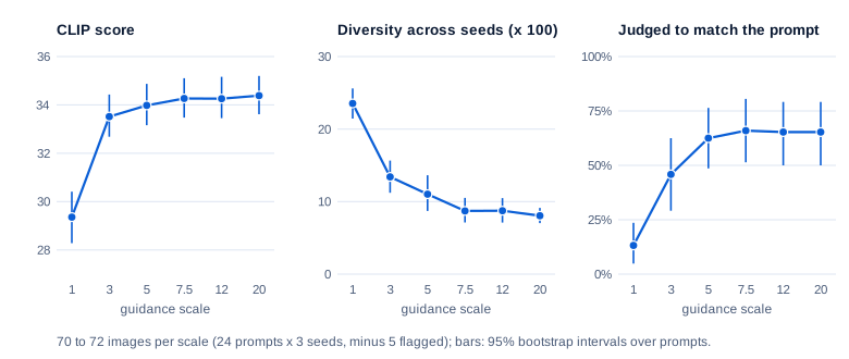
The sweep used 24 prompts written for this article (objects, animals, food and landscapes, most with a colour, count or arrangement to check, such as “three green apples on a white plate”), 3 seeds each and six guidance scales, 432 images at 512 × 512 with 20 DPM-Solver++ steps. Each image got three measurements:
- CLIP score: 100 times the cosine similarity of image and prompt as embedded by openai/clip-vit-base-patch32 (MIT license), a different CLIP from the one inside Stable Diffusion, so the generator isn’t grading itself. (Hessel et al., 2021 use a weight of 2.5 instead of 100.)
- Diversity: the average cosine distance (1 minus the similarity) between the CLIP image embeddings of a prompt’s 3 seeds.
- A judge: Claude Haiku 5.5 (
claude-haiku-5-5, thinking disabled, 16 output tokens at most) asked “Does the image show everything the caption asks for: each named object, its color, its number and how the objects are arranged?” with a one-word answer. All 491 judge requests, the negative-prompt test included, ran through the Batch API for $0.011. Five replies (1%) ran out of tokens while explaining and are left out.
Swipe to pan the diagram, or tap it to zoom.
Everything moves between 1 and 5, then stops. The CLIP score climbs 4.9 points from scale 1 to 7.5 (paired by prompt and seed, 3.9 to 5.8) and then 0.3 more by 20 (−0.1 to +0.7), no change this experiment can detect. Judged adherence rises from 13% to 63% at scale 5 and stays near 65%. Diversity falls by almost two thirds by 7.5.
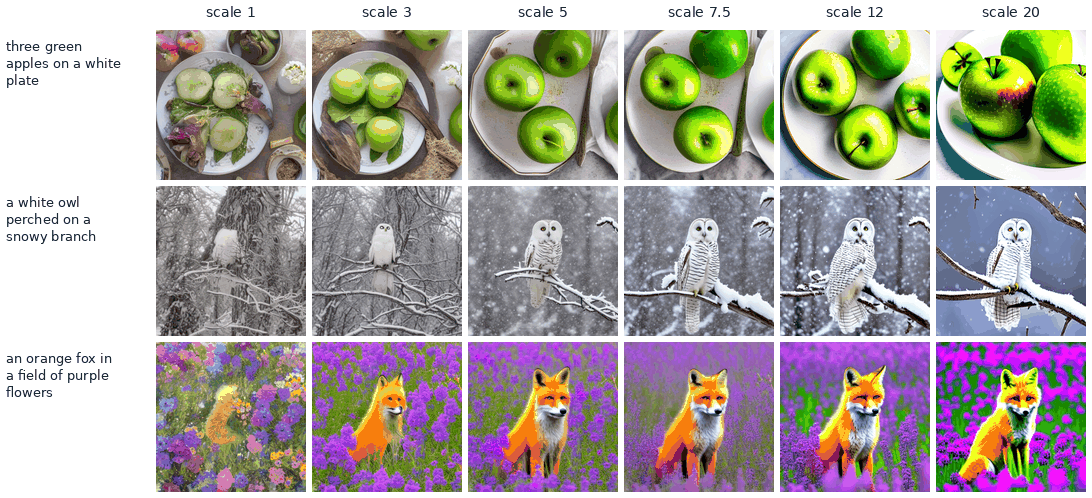
Past 7.5 the pictures just get louder. Mean colour saturation (the S channel of HSV, 0 to 1) rose from 0.24 at scale 1 to 0.43 at 7.5 and 0.57 at 20: extrapolating away from the unconditional image pushes colour and contrast as well as content.
Checking the judge
71 of the images (seed 11 at scales 1, 7.5 and 20, shuffled) were also labelled by hand, before seeing Haiku’s answers. Haiku agreed on 55 of 71, 77% (66 to 86), a Cohen’s kappa (agreement corrected for chance) of 0.55. It was the stricter grader: it rejected 13 images the hand labels accepted, against 3 the other way. The hand labels show the same shape: 22% (10 to 42) at scale 1, 75% (55 to 88) at 7.5 and 88% (69 to 96) at 20. The failures were the compositional ones the model card warns about: “a blue ceramic vase with yellow tulips” gave a yellow vase at 7.5, and “a giraffe standing next to a palm tree” a palm with a giraffe-patterned trunk.
Step 4: samplers, and why 20 steps are enough
Stable Diffusion was trained like Part 5’s model, with 1,000 noise levels (its scheduler config lists 1,000 training timesteps), yet it makes good images in 20 to 50 steps. The reason is the sampler, the rule that turns the U-Net’s noise prediction into the next latent. DDIM (Song, Meng and Ermon, 2020) showed that the same network can be sampled deterministically, adding no fresh noise and skipping most of the levels, for “high quality samples 10× to 50× faster.” Sampling then means solving an ordinary differential equation (ODE), a rule for how the latent changes as the noise falls. DDIM takes first-order steps: follow the current slope for a while. diffusers’ Euler sampler does the same in the noise-level parameterization of Karras et al. (2022). DPM-Solver++ (Lu et al., 2022) is a second-order solver for guided sampling: it works with the predicted clean image and reuses the previous step’s prediction to correct the current one, at no extra U-Net cost. Its paper says DDIM “generally needs 100 to 250 steps” with guidance and DPM-Solver++ “15 to 20 steps.”
Steps against a converged image
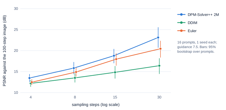
Each of 16 prompts ran with one seed and guidance 7.5, with all three samplers at 4, 8, 15 and 30 steps, plus a reference made with 100 DPM-Solver++ steps. All start from the same noise and approximate the same ODE, so all should approach the reference; the chart measures how close they get.
Swipe to pan the diagram, or tap it to zoom.
DPM-Solver++ is closest at every count, 23.1 dB (20.7 to 25.6) at 30 steps, though the reference is DPM-Solver++ too, which favours it. Euler closes in at 20.5 dB; DDIM, with diffusers’ default step spacing, moves slowly. PSNR punishes small shifts of edges and texture, and the content settles much sooner:
| Steps | DDIM | Euler | DPM-Solver++ | Time per image |
|---|---|---|---|---|
| 4 | 31.9 (30.6 to 33.3) | 32.9 (31.4 to 34.3) | 34.0 (32.8 to 35.3) | 0.64 s |
| 8 | 34.4 (33.3 to 35.7) | 34.5 (33.4 to 35.8) | 34.6 (33.5 to 35.9) | 1.09 s |
| 15 | 34.1 (32.7 to 35.7) | 34.3 (33.2 to 35.4) | 34.2 (33.0 to 35.6) | 1.87 s |
| 30 | 33.7 (32.7 to 34.8) | 34.6 (33.6 to 35.6) | 34.4 (33.4 to 35.6) | 3.5 s |
| 100 (reference) | 34.4 (33.3 to 35.6) | 11.6 s |
Cells are mean CLIP scores over the 16 prompts with bootstrap intervals; times are per image in batches of 4 (median over the 48 images per step count). From 8 steps on, every sampler matches the 100-step reference; only at 4 steps does DDIM fall behind. Deterministic samplers follow a smooth path, so large steps lose little, and higher-order solvers correct for its curvature. And, as the next figure shows, the layout is decided in the first few steps.
Watching the latent during sampling
Every noise prediction implies a guess at the finished latent: subtract the predicted noise, scaled for the current noise level, and you get the current estimate of the clean latent, written x0. Decoding it at each step shows the picture forming (DDIM, 20 steps, scale 7.5, “a lighthouse on a rocky cliff at sunset”, seed 11):
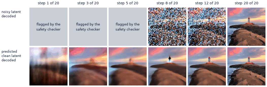
After step 1, at a signal-to-noise ratio of 0.008, the predicted clean latent already correlates 0.60 with the final one; by step 5, 0.86. The other 15 steps refine edges, colour and the lighthouse itself, as the prediction’s PSNR against the final picture climbs from 13.5 dB to 21.2 dB at step 5 and 31.4 dB at step 17.
Decoded directly, a noisy latent is coloured confetti, as the top row shows, and the safety checker flagged 17 of the 40 noisy latents decoded in this experiment (the first 7 to 10 steps of each run), against none of the 40 clean-latent predictions. The checker is a similarity threshold in CLIP space, and random textures can cross it.
In the real world
- SDXL (Podell et al., 2023) scaled the recipe: a 2.6B-parameter U-Net against 860M, and two text encoders (CLIP ViT-L and OpenCLIP ViT-bigG, 817M parameters together) with a 2,048-wide context instead of 768.
- Imagen (Saharia et al., 2022) used a frozen T5 language model as its text encoder and found “scaling the text encoder size to be significantly more impactful than the U-Net size”.
- The latent diffusion paper’s 1.45B-parameter text-to-image model scored an FID (Fréchet Inception distance, a distance between generated and real images in a classifier’s feature space; lower is better) of 23.31 on 256 × 256 MS-COCO without guidance and 12.63 with a scale of 1.5 (reported, not reproduced here).
- Distillation cuts the steps again: Latent Consistency Models (Luo et al., 2023) train a student in “∼32 A100 GPU Hours” that needs “2∼4 steps or even one step”, and Adversarial Diffusion Distillation (Sauer et al., 2023) gets down to 1 to 4 steps (both reported, not reproduced here).
- Newer models replace the U-Net with a transformer over patches of the latent and the noise-prediction objective with flow matching: Stable Diffusion 3 and FLUX, the subject of Part 7.
Common misconceptions
- “Stable Diffusion paints pixels.” The U-Net never sees one. It denoises a 4 × 64 × 64 latent, and the VAE decoder, run once at the end, invents the pixels. That’s one reason fine lettering comes out garbled: the latent has one cell per 8 × 8 pixels.
- “A higher guidance scale means a better image.” Judged adherence rose from 13% at scale 1 to 63% at 5 and stayed flat after, while seeds grew more alike and saturation rose by a third between 7.5 and 20.
- “More steps are always better.” At 8 steps every sampler’s CLIP score matched the 100-step reference (34.4 to 34.6 against 34.4), and 30 steps took 3.2 times as long. Extra steps sharpen pixels; the content is decided early.
- “A negative prompt is a filter that blocks things.” It replaces the empty prompt in the guidance formula, so the sampler steers away from that text. It removed red flowers from 4 of 4 gardens, and also rearranged fruit bowls that had no bananas to remove.
- “The safety checker makes the model safe.” It runs after the image exists, as a CLIP similarity test against 17 hidden concepts, and swaps flagged images for black ones. The model’s weights are unchanged.
Key takeaways
- Stable Diffusion denoises a 4 × 64 × 64 latent, not pixels: 803 GFLOP per U-Net pass, against 545,118 for the same network on pixels.
- A frozen CLIP text encoder, an 860M-parameter U-Net that reads the text by cross-attention, and a VAE decoder share the work; the U-Net takes 93% of the 2.77 seconds.
- Classifier-free guidance runs the U-Net with and without the prompt and extrapolates past the conditional prediction. It costs 1.6 times as much per step, and it lifted judged adherence from 13% to about 65%, with little gain past a scale of 5.
- A negative prompt is just the text in the unconditional branch: it can remove a concept, and it changes the rest of the picture too.
- With modern samplers the layout is fixed in the first quarter of the steps, and 8 steps matched a 100-step image’s CLIP score.
- The safety checker is a CLIP threshold applied afterwards: it flagged 5 of 704 harmless images, and 17 of 40 decoded noise latents.
What’s next
Part 7 replaces the U-Net and the noise-prediction objective: a diffusion transformer that cuts the latent into patches like the vision transformers of Part 2, and flow matching, which learns straight paths from noise to image so that even fewer steps are needed. It’s the design behind Stable Diffusion 3 and FLUX.
Further reading
- High-Resolution Image Synthesis with Latent Diffusion Models (Rombach et al., 2021): perceptual against semantic compression, cross-attention conditioning, and the cost argument.
- Classifier-Free Diffusion Guidance (Ho and Salimans, 2022): one network with and without the condition, and the guidance formula.
- Denoising Diffusion Implicit Models (Song, Meng and Ermon, 2020): deterministic sampling with far fewer steps.
- DPM-Solver++: Fast Solver for Guided Sampling of Diffusion Probabilistic Models (Lu et al., 2022): the second-order multistep sampler used for most images here.
- Elucidating the Design Space of Diffusion-Based Generative Models (Karras et al., 2022): sampling as an ODE, noise levels and Euler steps.
- Stable Diffusion v1-5 model card: training data, steps, text-condition dropping, limitations and the safety module.
- SDXL (Podell et al., 2023): how the same recipe scales to a 2.6B U-Net and two text encoders.
- CLIPScore (Hessel et al., 2021): the reference-free image-text score behind the CLIP score used here.
- Photorealistic Text-to-Image Diffusion Models with Deep Language Understanding (Saharia et al., 2022): Imagen, and why a bigger text encoder helps more than a bigger U-Net.
- Stable Diffusion with Diffusers (Hugging Face blog): a walk through the same three components with code.