
Beyond Text: Images, Speech and Video · Part 8 of 13
Autoregressive Image Generation: Drawing Pictures as Tokens
VQ tokenizers, raster-order and masked transformers, next-scale prediction and unified models: how LLM-style models draw images, measured on a laptop.
On this page
TL;DR
A language model can draw once a picture is turned into a short sequence of integer codes. This article builds that pipeline on a laptop: a small VQ-VAE that turns each Fashion-MNIST image into 49 codes, and two transformers that write those codes, one strictly in order and one that fills in many per pass, as MaskGIT does. It measures what the tokenizer loses, how many codebook entries get used, and how quality and speed change with the number of passes. Then it times aMUSEd, an open masked text-to-image model, and maps the newer designs: next-scale prediction, continuous tokens and unified models.
Why it matters
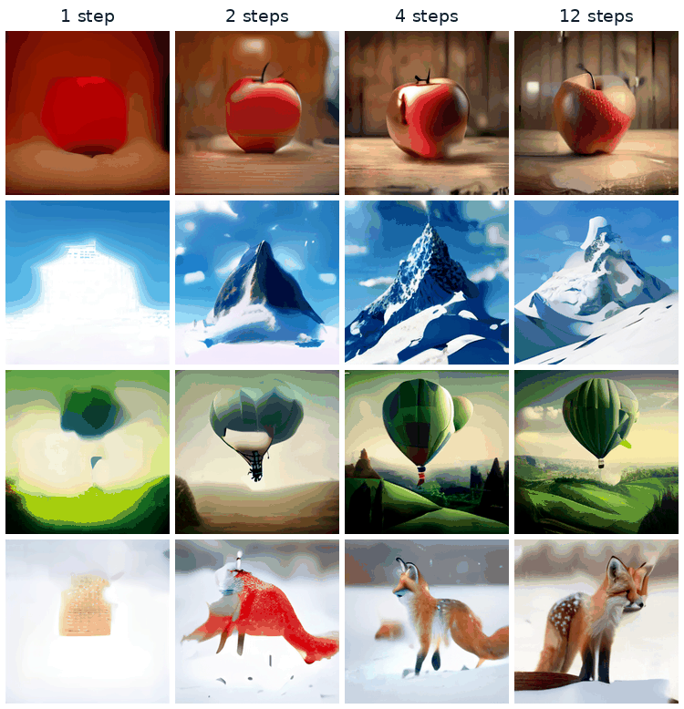
On a laptop GPU, a small transformer that writes a Fashion-MNIST picture one code at a time takes 139 ms and 49 passes per image. The same network trained to fill in many codes at once needs 8 passes and 26 ms, and the pictures come out worse, 37 against 15.5 on the quality score used here. Meanwhile aMUSEd, an open text-to-image model, draws a recognizable red fox in the snow from its prompt in 4 decoding steps and a quarter of a second.
OpenAI’s GPT-4o system card addendum says “unlike DALL·E, which operates as a diffusion model, 4o image generation is an autoregressive model natively embedded within ChatGPT.” That sentence is most of what is public about it. The open papers show how a picture becomes tokens, in which order to write them, and what each choice costs. Part 1 measured a real VQ-GAN tokenizer, 1,024 codes for a 512-pixel picture; this part generates with codes like those.
The intuition
Think of a mosaic made from a box of 512 tile designs. To copy a picture, you pick for each square the design that looks closest. To invent a picture, you only choose a design number for each square, and someone else glues the tiles down.
The box is the codebook, the design numbers are image tokens, and choosing them is the transformer’s job. A raster-order model is an apprentice filling squares left to right, top to bottom, never going back. A masked model is a master who places a few tiles it is sure of anywhere on the board, steps back, and fills in more each round.
The analogy breaks at the glue. The decoder is a neural network that blends neighbouring codes into smooth pixels, so a code means something slightly different next to different neighbours. And the box is learned along with the encoder and decoder, which is why some designs end up never used.
Step 1: turning a picture into tokens
The tokenizer is an autoencoder with a codebook in the middle. An encoder shrinks the image to a small grid of vectors, each vector is replaced by its nearest codebook entry, and a decoder turns the grid back into pixels. The image is then just a list of entry numbers. VQ-VAE (van den Oord et al., 2017) introduced this, compressing 128 × 128 ImageNet pictures into a 32 × 32 grid of codes from 512 entries.
Picking the nearest entry has no gradient, so training uses two tricks. The straight-through estimator copies the decoder’s gradient past the lookup to the encoder, as if the lookup weren’t there. And two terms join the reconstruction error: one pulls each used entry toward the encoder outputs assigned to it, and the commitment loss, weighted by β, pulls encoder outputs toward their entries. The paper found results “did not vary for values of β ranging from 0.1 to 2.0” and used 0.25. In code, with random numbers standing in for a real encoder’s output, the whole quantizer is a few lines:
import torch
import torch.nn.functional as F

torch.manual_seed(0)
z = torch.randn(49, 64, requires_grad=True)          # 7 x 7 encoder outputs, 64 numbers each
codebook = torch.randn(512, 64, requires_grad=True)  # 512 learned entries
dist = (z ** 2).sum(1, keepdim=True) - 2 * z @ codebook.T + (codebook ** 2).sum(1)
idx = dist.argmin(1)                                 # the image tokens: 49 integers
zq = codebook[idx]
vq_loss = F.mse_loss(zq, z.detach()) + 0.25 * F.mse_loss(z, zq.detach())  # codebook + commitment
zq = z + (zq - z).detach()                           # straight-through: forward uses zq, gradient reaches z
print(idx.shape, idx[:6].tolist())
# torch.Size([49]) [491, 16, 108, 499, 7, 501]
What a small tokenizer keeps
The tokenizer here has two stride-2 convolutions down, two residual blocks, 64-number code vectors and the mirror image up: 7 × 7 codes for a 28 × 28 image. It trained on the 60,000 Fashion-MNIST training images (Zalando Research, MIT license; Xiao et al., 2017) for 3,000 steps of 256 images with plain mean-squared error, about a minute on the laptop’s RTX 4060. Quality is scored with FD-FMNIST, a Fréchet distance between features of generated and real images taken from our own small Fashion-MNIST classifier, not the Inception network behind published FID scores, so it only compares our models with each other. Lower is better: 5,000 real training images score 0.64 against the test set, the same images blurred 73.8, uniform noise 718.
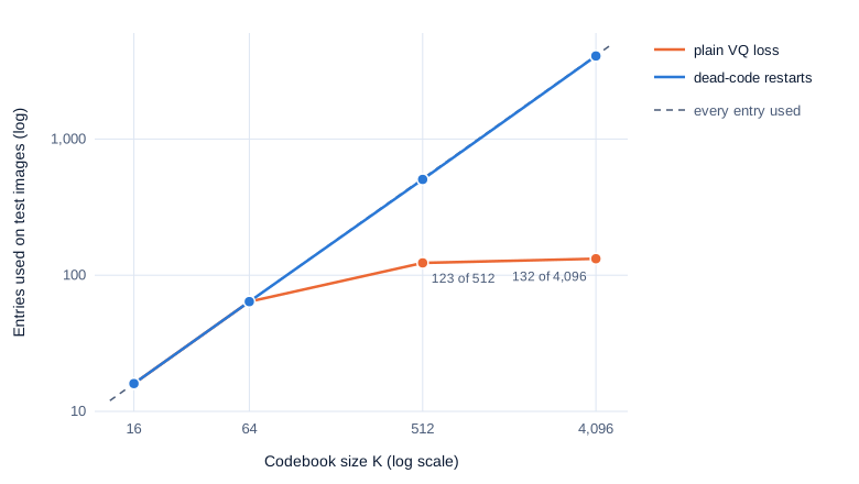
Two numbers describe the codebook. Entries used counts how many of the K entries appear at least once on the 10,000 test images. Perplexity, the exponential of the entropy of how often each entry is used, is the number of entries that would give the same spread if all were used equally. One training seed per row:
| Entries K | Dead-code restarts | Entries used | Perplexity | Error (MSE) | PSNR | FD-FMNIST of 5,000 reconstructions |
|---|---|---|---|---|---|---|
| 16 | no | 16 | 10.9 | 0.032 | 21.0 dB | 13.4 |
| 64 | no | 64 | 36.5 | 0.024 | 22.2 dB | 11.9 |
| 512 | no | 123 | 85.5 | 0.024 | 22.3 dB | 8.6 |
| 4,096 | no | 132 | 92.6 | 0.028 | 21.5 dB | 13.4 |
| 16 | yes | 16 | 12.3 | 0.031 | 21.1 dB | 12.8 |
| 64 | yes | 64 | 49.0 | 0.030 | 21.2 dB | 16.8 |
| 512 | yes | 505 | 420 | 0.025 | 22.0 dB | 16.2 |
| 4,096 | yes | 4,071 | 3,350 | 0.032 | 20.9 dB | 25.6 |
The error is the mean squared difference per pixel on the [-1, 1] scale; PSNR (peak signal-to-noise ratio) is the same error on a log scale, higher is better. At 512 entries an image’s 49 codes hold 49 × 9 = 441 bits, 14 times fewer than its 784 raw 8-bit pixels.
Swipe to pan the diagram, or tap it to zoom.
With the plain loss, the codebook collapsed: past 64 entries, only 123 of 512 and 132 of 4,096 were ever used. An entry that no encoder output lands near gets no gradient, never moves toward the data, and stays dead. The simplest fix: every 200 steps, move each entry unused in that window onto a random encoder output from the current batch. With it, 505 of 512 and 4,071 of 4,096 entries stayed alive.
Live entries didn’t make better pictures, though. Error barely moved from 64 entries up, and the restarted large codebooks scored worse on FD-FMNIST, plausibly because entries kept being thrown to new places with only 3,000 steps to settle. With one seed per row, a few FD points may be noise; two sets of 5,000 reconstructions from the same tokenizer scored 8.6 and 8.9.
The grid mattered far more. With one stride-2 layer instead of two, 14 × 14 = 196 codes and 512 entries with restarts, 4,000 steps reached an error of 0.0077, 27.2 dB and an FD-FMNIST of 4.0, against 0.024, 22.2 dB and 13.6 for 7 × 7 with identical settings. Four times the codes cut the error 3.1 times, and quadrupled the sequence a prior must write. The priors below use the 7 × 7, 512-entry tokenizer without restarts, the best row above, to fit the laptop’s time budget.
VQGAN: losses that care what an image looks like
Mean-squared error rewards blur, because when the decoder can’t tell where an edge goes, averaging the options scores best. VQGAN (Esser et al., 2020) kept the codebook and changed the loss: “we replace the L2 loss … by a perceptual loss and introduce an adversarial training procedure with a patch-based discriminator.” The perceptual loss compares images in a pretrained network’s feature space instead of pixel by pixel. The discriminator, a second network, learns to tell real patches from reconstructed ones, and the decoder learns to fool it, which pushes it toward sharp, plausible texture. A weight λ, set from the two losses’ gradients at the decoder’s last layer, balances them.
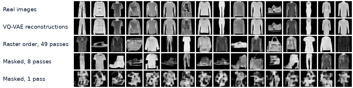
That’s what lets VQGAN shrink each side 16 times and still hand a transformer something worth generating. Its ImageNet model still used only part of its codebook: “k = 973 is the effective size of the VQGAN’s codebook” of 16,384 entries. LlamaGen (Sun et al., 2024) later cut the code vectors to 8 numbers, normalized them, and reports “codebook usage of 97%” for 16,384 entries. Both reported, not reproduced here. The small tokenizer above uses MSE only, which is why its reconstructions in the sample grid below are soft.
Step 2: one token at a time
Once images are codes, generating them is language modeling. Flatten the 7 × 7 grid in raster order, row by row like text, and train a transformer to predict each code from the ones before it with a language model’s cross-entropy loss (Math Part 4). To sample, feed a start token, draw code 1, feed it back, draw code 2, and so on, 49 times.
DALL-E (Ramesh et al., 2021) did this at scale: a 12-billion-parameter transformer over “up to 256 BPE-encoded text tokens” followed by “32 × 32 = 1024 image tokens” from an 8,192-entry codebook, trained on 250 million image-text pairs. Its tokenizer “reduces the context size of the transformer by a factor of 192”, and each published sample was “the best of 512 as ranked by” CLIP (Part 3). Parti (Yu et al., 2022) scaled the recipe to 20 billion parameters with a ViT-VQGAN tokenizer, reaching a zero-shot MS-COCO FID of 7.23. LlamaGen used the Llama language-model architecture with no image-specific design, “vanilla autoregressive models” in its words, and reports ImageNet 256 × 256 FID 2.18 for its 3.1B model with classifier-free guidance (sampled at 384 pixels and resized). All reported, not reproduced here.
The raster-order prior, measured
The prior is a 6-layer transformer, width 256, 5.0M parameters, trained on the training images’ codes for 2,500 steps of 256 sequences (about 11 full sweeps of the data) in bfloat16: 121 seconds. On the test codes its loss was 1.98 nats per code, against 4.8 for a uniform guess among the 123 codes in use.
Sampled at temperature 1.0, 5,000 images scored an FD-FMNIST of 15.5 (15.2 to 15.9 across three sampling seeds). The tokenizer’s reconstructions of real images score 8.95 at the same sample size and real images 0.64. No prior over these codes can beat 8.95: its best possible output is a perfect copy of the code distribution, which the decoder softens the same way. Temperature 0.9, favoring likelier codes, scored worse, 22.8: less varied images, with sneakers 16.7% of the time instead of about 10%.
The cost is the loop: one pass per code, 49 per image. Timed on the NVIDIA GeForce RTX 4060 Laptop GPU (8 GB) with PyTorch 2.11, median of 7 runs after 3 warm-ups with torch.cuda.synchronize() around each, and the clock and power read with nvidia-smi during the runs:
| Sampler | Passes per image | One image | Batch of 500: images per second |
|---|---|---|---|
| Raster order, KV cache | 49 | 139 ms | 1,740 |
| Raster order, no cache | 49 | 132 ms | 660 |
| Masked, 4 passes | 4 | 14 ms | 3,760 |
| Masked, 8 passes | 8 | 26 ms | 1,960 |
| Masked, 16 passes | 16 | 53 ms | 1,000 |
Images per second include the decoder, 8 ms per 500 images. A KV cache keeps the attention keys and values of codes already written, so each pass computes only the newest position (Inference Part 2). For one image it saved nothing: 49 tiny passes leave the GPU idling at 1,620 MHz and 12 W, waiting on kernel launches. For 500 at once, at 2,175 MHz and 41 W, it made sampling 2.6 times faster.
Step 3: many tokens per pass
Raster order commits to the top-left corner before the picture is decided, one pass per token. MaskGIT (Chang et al., 2022) trains the same transformer differently: a random share of each image’s codes, drawn from a cosine schedule, is replaced by a [MASK] token, and the model, attending in both directions, predicts the hidden codes from the visible ones.
To sample, start fully masked. Each pass predicts every masked position, keeps the most confident predictions and re-masks the rest, leaving N × cos(π/2 × t/T) masked after pass t of T. With 49 codes and 8 passes, the passes reveal 1, 3, 5, 6, 7, 9, 9 and 9 codes: a cautious start, then bigger bites. The ranking gets randomness “with temperature annealing to encourage more diversity”, and the paper found cosine the best schedule, with “the earliest sweet spot at a total of 8 to 12 iterations.” It reports ImageNet 256 FID 6.18 in 8 passes, and that it “accelerates autoregressive decoding by up to 64x”.
The masked prior, measured
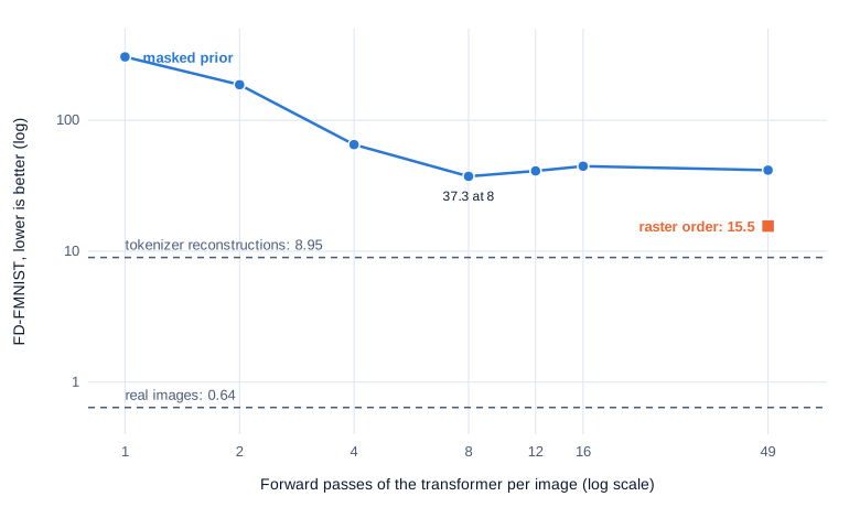
The masked prior is the same network with the causal mask removed, trained for the same 2,500 steps. Scored the same way:
Swipe to pan the diagram, or tap it to zoom.
One pass is hopeless, 304: every code is drawn at once from its own distribution, with nothing to agree with. Each doubling up to 8 passes roughly halved the score, and 8 was the sweet spot, 37.3 (37.2 to 37.3 across seeds). At 8 passes the masked prior made an image in 26 ms, 5.4 times faster than raster order, and still lost on quality by more than a factor of two.
The ranking rule explains part of that. The codes a model is most sure of are the easy ones: background cells and the outlines of the simplest garments. A second run varied only the Gumbel noise added to the ranking:
| Ranking noise | 8 passes | 49 passes, one code each |
|---|---|---|
| None: pure confidence | 472 | 680 |
| Scale 1 | 235 | 222 |
| Scale 4.5 (used above) | 37.3 | 41.5 |
| Huge: effectively random order | 45.0 | 35.2 |
Mean of 3 seeds of 5,000 samples each; every spread was under 8 points. With pure confidence ordering the prior collapsed: among 5,000 samples the classifier found no pullovers, coats or shirts, and 36% sandals. Noise breaks the collapse. Yet even in random order with one code per pass, the masked prior reached only 35, against 15.5 for raster order with the same 49 passes. The rest of the gap is what it learned. A raster model learns one ordering and gets a target at all 49 positions of every training sequence. A masked model must handle any subset of known codes and gets targets only at the masked share, 64% on average under the cosine schedule. In the same 2,500 steps that is a harder job with less signal; MaskGIT trained far longer, on ImageNet.
Batch size changes the timing picture. With 500 images at once the GPU is busy, and total work counts more than the number of passes. Raster order with a KV cache computes each of the 49 positions once; masked decoding recomputes all 49 in every pass, 392 position-computations in 8 passes. So it made 1,960 images per second against raster order’s 1,740: fewer passes cut the wait for one image much more than they raise throughput.
Muse and aMUSEd: masked generation from text
Muse (Chang et al., 2023) put text in front of MaskGIT: a frozen T5-XXL text encoder, a base model writing 16 × 16 codes in 24 passes, and a super-resolution model writing 64 × 64 codes in 8 more. It reports a zero-shot COCO FID of 7.88 for its 3B model, and “each image was generated in 1.3s on a TPUv4 chip”. aMUSEd (Patil et al., 2024) is the open reproduction: a CLIP-L/14 text encoder, a 146M-parameter VQ-GAN that shrinks each side 16 times into 8,192 codes, and a 603M-parameter U-ViT (a transformer with convolutional blocks around it) for the 256-pixel model, “800M” in all, using 12 decoding steps.
amused/amused-256 (OpenRAIL++ license, ungated; 1.75 GB of fp16 weights) ran in float16 with the VQ-GAN in float32, as its model card advises. It ships with no safety checker; the prompts describe objects, animals, food, buildings, landscapes and abstract patterns, no people. By default it uses classifier-free guidance at scale 10 (Part 6 explains it): each pass runs the transformer with and without the prompt and extrapolates from the difference.
The test: 40 prompts, seeds 0, 1 and 2, 256 × 256 pixels, default guidance and scheduler, 1 to 24 decoding steps. Alignment is scored with a different CLIP than the one inside aMUSEd, CLIP ViT-B/32 (Part 3): the CLIP score is 100 times the cosine similarity of image and prompt embeddings. Scoring each image against the 39 other prompts gives a mismatch baseline, and the share of images whose own prompt beats all 39 others says whether the picture shows what was asked. Intervals are 95% bootstrap intervals over prompts for the score and Wilson intervals for the share.
| Decoding steps | Transformer runs | Time per image | CLIP score (95% CI) | Mismatched prompts | Own prompt ranked first of 40 |
|---|---|---|---|---|---|
| 1 | 2 | 129 ms | 23.7 (22.5-24.8) | 18.3 | 36% (28-45) |
| 2 | 4 | 169 ms | 29.4 (28.5-30.2) | 16.4 | 87% (79-92) |
| 4 | 8 | 253 ms | 31.4 (30.7-32.1) | 15.2 | 99% (95-100) |
| 8 | 16 | 416 ms | 31.8 (31.2-32.5) | 15.0 | 99% (95-100) |
| 12 (default) | 24 | 581 ms | 31.6 (30.9-32.4) | 14.9 | 100% (97-100) |
| 16 | 32 | 757 ms | 31.7 (30.9-32.4) | 15.0 | 99% (95-100) |
| 24 | 48 | 1,090 ms | 31.8 (31.1-32.6) | 14.9 | 99% (93-100) |
Each row holds 120 images, except 24 steps, where the run hit its time limit after two seeds (80 images). Times are for one image, median of 7 runs after 3 warm-ups, at 2,025 to 2,175 MHz and 38 to 41 W.
Alignment stopped improving at 4 steps. Paired by prompt, 4 steps scored 0.27 points below 12 (95% CI -0.61 to +0.06), and 8, 16 and 24 steps were within 0.2 of it. One step gives a blurry color field that names its prompt 36% of the time; two steps give the right object with rough edges. Later steps add detail and texture that CLIP ViT-B/32 doesn’t reward, so this measures alignment, not overall quality. The paper reports a zero-shot COCO FID of 38.7 and CLIP score of 25.97 for this model at 12 steps, on its own setup; not reproduced here.
Of the 581 ms, the text encoder takes 4.6 ms (prompt plus empty negative prompt), each transformer pass on that batch of two 39 ms, and the float32 VQ-GAN decoder 66 ms: the twelve passes are 80%. Guidance doubles the batch but barely the time; without it, 12 steps took 561 ms, because one 256-code image doesn’t fill the GPU. Eight prompts at once took 3.27 s, 408 ms per image. The paper reports 0.47 s per image at batch 1 on an A100; the laptop took 24% longer.
Diffusion, flow and tokens on one scale
Part 5 and Part 7 scored diffusion and flow models on the same FD-FMNIST metric. The networks, sizes and training budgets differ, so this is a rough lineup, not a controlled race:
| Approach | Network and training | Passes per image | FD-FMNIST (samples) |
|---|---|---|---|
| Diffusion, DDIM sampler (Part 5) | 1.59M-parameter U-Net, 11,500 steps | 50 | 5.66 (5,000) |
| Diffusion, DDIM sampler (Part 7) | 4.10M-parameter U-Net, 4,000 steps | 32 | 9.3 (2,000) |
| Rectified flow, Euler steps (Part 7) | the same U-Net, 4,000 steps | 32 | 9.1 (2,000) |
| Rectified flow after reflow (Part 7) | the same U-Net, fine-tuned | 1 | 46.5 (2,000) |
| Raster-order prior over VQ codes | 5.0M-parameter transformer, 2,500 steps | 49 | 15.5 (5,000) |
| Masked prior over VQ codes | the same transformer, 2,500 steps | 8 | 37.3 (5,000) |
Real images score 0.64 with 5,000 samples and 1.05 with 2,000. The token models trail mainly because of their tokenizer: no prior over these 7 × 7 codes can score below the 8.95 of its own reconstructions, while the diffusion and flow models write pixels directly. At a similar number of passes, the raster prior’s 15.5 sits between that floor and the pixel models’ 6 to 9.
Step 4: changing what a step predicts
Raster order and masking both predict codes on one fixed grid. Two newer designs change the unit of prediction instead.
Next-scale prediction
VAR (Tian et al., 2024) recasts autoregression on images as “coarse-to-fine ‘next-scale prediction’”. Its tokenizer encodes an image as a stack of code maps of growing resolution from one shared 4,096-entry codebook. Generation “is then started from the 1×1 token map, and progressively expands in resolution”, each step predicting a whole map from all the coarser ones: 10 steps for a 256 × 256 image.
That answers both complaints about raster order. The layout is decided first and the detail later, and the number of passes follows the number of scales, not codes. The paper reports ImageNet 256 FID improving “from 18.65 to 1.73” over its raster baseline “with 20× faster inference speed” (the 1.73 is a 2.0B-parameter model with rejection sampling), and “clear power-law scaling laws similar to those observed in LLMs”. Reported, not reproduced here.
Continuous tokens
Every model so far pays the quantization tax measured in Step 1. MAR (Li et al., 2024) drops the codebook. Its transformer “autoregressively predicts a vector z for each token, which serves as a conditioning for a denoising network (e.g., a small MLP)” trained with a diffusion loss. The transformer decides what goes where, and a tiny per-token diffusion model supplies exact numbers no codebook has to contain. It predicts sets of tokens in random order, as MaskGIT does, and its 943M-parameter model reports ImageNet 256 FID 1.55 with classifier-free guidance, at under 0.3 seconds per image on an A100 at batch 256 for an FID under 2.0. Reported, not reproduced here.

Mostly the prior’s decoding loop differs between designs, though VAR also needs a tokenizer that writes one code map per scale.
In the real world
The same machinery now sits inside models that also read. Fundamentals Part 15 introduced early fusion; here is how unified models write images. Results are reported by the papers, not reproduced here.
| Model | How it writes an image | Size | Reported result |
|---|---|---|---|
| Chameleon (Meta, 2024) | 1,024 VQ codes per 512 × 512 image from 8,192 entries, in one vocabulary with text | 7B, 34B | 34B preferred over Gemini-Pro in 60.4% of human pairwise comparisons |
| Transfusion (Meta, 2024) | Continuous VAE patches, denoised by diffusion inside the same transformer | 7B | COCO FID 6.78, GenEval 0.63 |
| Janus (DeepSeek, 2024) | VQ codes from 16,384 entries for writing; separate SigLIP features for reading | 1.3B | GenEval 0.61 |
| Emu3 (BAAI, 2024) | 4,096 codes per 512 × 512 image from 32,768 entries | 8B | Says it surpasses SDXL and LLaVA-1.6 |
| GPT-4o image generation (OpenAI, 2025) | Undisclosed beyond “an autoregressive model” | Undisclosed | None in the addendum |
- Chameleon trained one transformer “from scratch” on about 10 trillion tokens of mixed text and images, and needed query-key normalization and a z-loss (a penalty on large softmax normalizers) to keep training stable.
- Transfusion keeps image patches continuous: next-token loss on text, diffusion loss on patches, one set of weights. It reports that it “exceeds the Chameleon approach at less than a third of the compute”.
- Janus reads with SigLIP features (Part 3) and writes with VQ codes, on the argument that understanding and generation want different encodings.
- For GPT-4o, the system card addendum says the generator is “autoregressive” and “embedded natively, deep in the architecture of our omnimodal GPT-4o model”. It doesn’t say what the tokens are or whether a diffusion decoder makes the pixels; anything more specific is inference.
Common misconceptions
- “Autoregressive image models must generate one token at a time.” Raster order does: 49 passes here, 1,024 for DALL-E. MaskGIT fills many codes per pass and VAR a whole resolution, each step conditioned on earlier ones.
- “A bigger codebook means sharper images.” Here, going from 64 to 4,096 entries didn’t lower reconstruction error, and without restarts the model used only 132 of 4,096 entries. Grid resolution mattered far more: 14 × 14 codes cut the error 3.1 times.
- “The transformer decides image quality.” It can’t beat its tokenizer. The best prior here scored 15.5; its tokenizer’s reconstructions, a floor no prior over those codes can beat, scored 8.95.
- “Fewer passes is always worse.” For the masked prior, 8 passes scored 37.3 and 16 passes 44.5. MaskGIT reports the same shape on ImageNet, with a sweet spot at 8 to 12 iterations.
- “GPT-4o’s image generator is known to work like Chameleon.” OpenAI’s published material says “autoregressive” and nothing about tokens or decoders.
Key takeaways
- A VQ tokenizer turns an image into a short grid of integers, and from then on generation is language modeling with a different vocabulary.
- The tokenizer sets the ceiling. The 7 × 7 tokenizer’s reconstructions scored 8.95 on FD-FMNIST, real images 0.64, and the best prior trained on its codes 15.5.
- Codebooks collapse without help: with the plain loss, a 4,096-entry codebook used 132 entries; restarting dead entries kept 99% alive, though at this scale that didn’t improve the pictures.
- Masked decoding traded quality for latency: 8 passes made an image 5.4 times faster than 49 raster passes but scored 37.3 against 15.5. At batch 500, the KV cache made raster order nearly as fast.
- aMUSEd draws a 256-pixel image from text in 0.58 s on a laptop GPU with 12 decoding steps, each one two transformer runs because of guidance.
- Newer designs change the unit of prediction (VAR) or drop the codebook (MAR); unified models put it all inside one transformer that also reads.
What’s next
That closes the image-generation half of the series. Part 9 turns to sound: how Whisper turns audio into log-mel spectrograms, why it is an encoder-decoder rather than a decoder-only model, and what its word error rate turns out to be when measured on a laptop.
Further reading
- Neural Discrete Representation Learning (van den Oord et al., 2017): VQ-VAE, the codebook, the straight-through estimator and the commitment loss.
- Taming Transformers for High-Resolution Image Synthesis (Esser et al., 2020): VQGAN’s perceptual and adversarial losses, and a transformer over its codes.
- Zero-Shot Text-to-Image Generation (Ramesh et al., 2021): DALL-E, text and image tokens in one autoregressive sequence.
- Scaling Autoregressive Models for Content-Rich Text-to-Image Generation (Yu et al., 2022): Parti, raster-order generation scaled to 20B parameters.
- Autoregressive Model Beats Diffusion: Llama for Scalable Image Generation (Sun et al., 2024): LlamaGen, a plain language-model architecture with a better tokenizer.
- MaskGIT: Masked Generative Image Transformer (Chang et al., 2022): parallel decoding with a cosine mask schedule.
- Muse: Text-To-Image Generation via Masked Generative Transformers (Chang et al., 2023) and aMUSEd: An Open MUSE Reproduction (Patil et al., 2024): masked generation from text, and the open model timed here.
- Visual Autoregressive Modeling: Scalable Image Generation via Next-Scale Prediction (Tian et al., 2024): VAR, one resolution per step.
- Autoregressive Image Generation without Vector Quantization (Li et al., 2024): MAR, continuous tokens with a per-token diffusion loss.
- Chameleon (Chameleon Team, 2024), Transfusion (Zhou et al., 2024), Janus (Wu et al., 2024) and Emu3 (Emu3 Team, 2024): four ways to read and write images in one transformer.
- Addendum to GPT-4o System Card: Native image generation (OpenAI, 2025): the one-sentence public description of GPT-4o’s image generator.
- Fashion-MNIST (Xiao et al., 2017): the dataset used for the experiments.
- amused/amused-256 model card (Hugging Face): weights, license and usage notes for the model timed here.