
Beyond Text: Images, Speech and Video · Part 7 of 13
Diffusion Transformers and Flow Matching: Straight Paths, Measured
How flow matching learns straight paths from noise to images, why reflow makes one step work, and what a DiT changes, measured on a laptop GPU.
On this page
TL;DR
Stable Diffusion 3 and FLUX.1 are rectified flow transformers: they learn a velocity along a straight line from noise to image (flow matching), and they replace the U-Net denoiser with a vision transformer over latent patches (a DiT). Trained on Fashion-MNIST on a laptop GPU with the same network and compute as a DDPM baseline, straight training paths alone sampled no better than diffusion with DDIM. One round of reflow, which straightens the learned paths, cut the error of a one-step sample from 724 to 46. At this small scale a tiny DiT lost clearly to a U-Net of the same size, because DiT’s advantage comes with scale and compute.
Why it matters
Ask a diffusion model for an image in one step and you get noise. Ask the rectified flow model trained here and you get a gray blob, the average of every garment it saw. Then fine-tune that same flow model for two minutes on 20,000 of its own outputs, and one step gives a recognizable shirt, shoe or bag. On the distance metric used here, the score drops from 724 to 46.5, where real images score 1.05.
Steps are what you pay for. Each sampling step is one full pass through the network, so 32 steps cost 32 times as much as one. The example on the Stable Diffusion 3.5 Large model card runs 28 steps; FLUX.1 [schnell] advertises “1 to 4 steps”. Fundamentals Part 15 sketched how diffusion models generate images and Part 1 measured the latents they work in. This part tests the two design choices behind the current generation: straight paths from noise to data, and a transformer backbone.
The intuition
Picture driving across a huge field toward one of several villages, allowed only a few glances at a compass. Between glances you drive straight. If the road from your start to your village is straight, one glance is enough. If it bends, every glance you skip takes you further off the road, and with a single glance you end up in an empty field halfway between two villages.
A sampler works the same way. It starts from pure noise, asks the network which way to move (one network call, one glance), takes a straight step, and repeats. The network’s answers define a set of roads from noise to images. Diffusion’s roads bend. Flow matching trains the network so that, as far as possible, they don’t.
The analogy breaks in one place. Flow matching trains on straight roads, one per pair of noise and image, but the roads the trained network follows still bend: from any point it sees many training roads crossing and can only point along their average. Straightening them takes an extra step, called reflow.
Step 1: flow matching draws straight lines
One pixel, worked by hand
Take one pixel. In the training image it is light gray, 0.6 on a scale from −1 to 1. The noise drawn for it is −1.2. Rectified flow (Liu et al., 2022) and flow matching (Lipman et al., 2022), two papers posted a month apart, join the two values with a straight line. Training picks a random time t between 0 (noise) and 1 (image):
x_t = (1 - t) * noise + t * image
t = 0.25:   x_t = 0.75 * (-1.2) + 0.25 * 0.6 = -0.75
target velocity:  v = image - noise = 0.6 - (-1.2) = 1.8
The network sees x_t and t and must output 1.8, the velocity along the line, which is the same at every point on it. The loss is the mean squared error against that target.
Generating means solving an ordinary differential equation (ODE), an equation for how fast something changes at each moment: dx/dt = v(x, t). The simplest solver is Euler’s method, x ← x + v(x, t) × Δt, one network call per step. On a perfectly straight road, one step of size 1 gives −1.2 + 1.8 = 0.6, the image exactly.
The catch is in “the network sees x_t”. At t = 0 the input is pure noise, and any training image could sit at the end of its line, so the best the network can do is output the average velocity, which points at the mean image. One Euler step from noise gives a blurry average of everything. In Liu et al.’s CIFAR-10 experiments one step scored an FID (Fréchet Inception Distance, a comparison of feature statistics of generated and real images; lower is better) of 378, against 2.58 for a full adaptive ODE solver taking 127 network calls (reported by Liu et al., not reproduced here).
The whole training step
Here is the training step and the sampler used in every experiment below, trimmed from this part’s lab module (which adds bf16 autocast). model(x, t) is any network that maps an image-shaped tensor and a batch of times to an image-shaped output.
import torch
import torch.nn.functional as F

def flow_loss(model, x1):                       # x1: a batch of images in [-1, 1]
    x0 = torch.randn_like(x1)                   # noise
    t = torch.rand(x1.shape[0], device=x1.device)
    tt = t[:, None, None, None]
    xt = (1 - tt) * x0 + tt * x1                # a point on the straight line
    return F.mse_loss(model(xt, t), x1 - x0)    # predict the velocity

@torch.no_grad()
def euler_sample(model, z, steps):              # z: noise, same shape as the images
    x, ts = z, torch.linspace(0, 1, steps + 1, device=z.device)
    for k in range(steps):
        x = x + (ts[k + 1] - ts[k]) * model(x, ts[k].expand(len(x)))
    return x
There is no table of noise levels, unlike Part 5’s DDPM with its 1,000-level schedule and DDIM update rule.
Same family as diffusion
Diffusion and flow matching both mix an image with noise as x_t = a × image + b × noise and train a network to undo the mix. DDPM uses a = sqrt(ᾱ) and b = sqrt(1 − ᾱ), where ᾱ (alpha-bar) is the share of signal left at that noise level. Since a² + b² = 1, the pair (a, b) moves along a quarter circle from (0, 1) to (1, 0). Rectified flow uses a = t and b = 1 − t, the straight line between the same two points.
DDPM predicts the noise and rectified flow the velocity, and either converts into the other. Lipman et al. showed both are special cases of one recipe, and their straight “optimal transport” path won on every dataset they tried: on ImageNet at 64 × 64, FID 14.45 with 138 network calls against 17.36 with 264 for DDPM (reported by Lipman et al., not reproduced here). For one image and noise pair, the quarter circle is π/2 ≈ 1.571 long against a chord of √2 ≈ 1.414, 11% longer before any learning happens. Keep that 1.11 in mind for Step 3.
Which times to train on
Esser et al. (2024), the Stable Diffusion 3 paper, compared 61 formulations with the same model and samplers. Near t = 0 the target is almost the dataset mean and near t = 1 the input is almost the image, so both ends are easy. Drawing t from a logit-normal distribution, t = sigmoid(u) with u normal, concentrates training on the middle. That variant, rf/lognorm(0.00, 1.00), “consistently achieves a good rank”, and “only rectified flow formulations with modified timestep sampling perform better” than the eps/linear formulation of earlier latent diffusion models. Plain rectified flow did not: at 25 steps on ImageNet it scored FID 49.70 against 48.42 for eps/linear and 45.78 for logit-normal (reported by Esser et al., not reproduced here). Step 2 finds the same on Fashion-MNIST.
Step 2: fewer steps, measured
The setup
Two copies of one network were trained on the 60,000 Fashion-MNIST training images (Xiao et al., 2017, MIT license, Zalando Research), 28 × 28 grayscale clothing in 10 classes. The network is a 4.10-million-parameter U-Net: a convolutional network that shrinks the image to 7 × 7 and grows it back, with skip connections, self-attention at 7 × 7, and the time added to every block. One copy learned DDPM noise prediction (linear schedule, 1,000 levels), the other rectified flow with uniform t. Both got 4,000 steps of batch 128 (8.5 passes over the data) with AdamW at 3e-4, bf16, and an exponential moving average (EMA) of the weights for sampling. Each run took about 6 minutes on an NVIDIA GeForce RTX 4060 Laptop GPU (8 GB, PyTorch 2.11, CUDA 12.8) at a median SM clock of 1,995 MHz and 44 to 46 W, with clocks and power limits at their defaults.
The metric is FD-FMNIST: the Fréchet distance (the formula behind FID) between features of generated images and the 10,000 test images, where the features come from a small classifier trained on Fashion-MNIST (91.1% test accuracy) instead of Inception. Its numbers are comparable only with each other, not with published FID. For scale, 2,000 real training images score 1.05, 5,000 real images blurred with a 3 × 3 box filter 73.8, and uniform noise 718. Every point below is the mean of 3 seeds of 2,000 samples, with the same starting noise for every model and step count.
DDIM and Euler tie
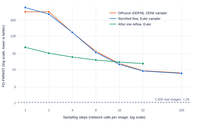
Swipe to pan the diagram, or tap it to zoom.
| Sampling steps | Diffusion, DDIM | Rectified flow, Euler | After one reflow, Euler |
|---|---|---|---|
| 1 | 541 (538 to 543) | 724 (723 to 724) | 46.5 (45.4 to 47.6) |
| 2 | 539 (536 to 541) | 460 (457 to 463) | 31.1 (29.8 to 32.1) |
| 4 | 130 (127 to 133) | 130 (128 to 133) | 23.8 (22.5 to 24.9) |
| 8 | 35.2 (34.4 to 35.6) | 32.7 (31.2 to 34.2) | 19.4 (18.0 to 20.7) |
| 16 | 15.3 (15.1 to 15.5) | 14.4 (13.5 to 14.9) | 16.8 (15.3 to 18.0) |
| 32 | 9.3 (9.1 to 9.5) | 9.1 (8.3 to 10.1) | 15.2 (13.8 to 16.2) |
| 100 | 8.0 (7.6 to 8.4) | 7.7 (7.0 to 8.8) | not run |
Brackets give the lowest and highest of the 3 seeds. From 4 steps on, rectified flow and diffusion stay within their seed ranges of each other: straight training paths did not, on their own, buy fewer steps. That matches Esser et al.’s 1.3-point gap at 25 steps. DDIM is itself “the Euler integration for a particular ODE” (Song et al., 2020), and that ODE’s paths are already fairly smooth.
At 1 and 2 steps both fail, differently. A single DDIM step divides by the remaining signal, sqrt(ᾱ) = 0.0064 at the noisiest level, so every error in the predicted noise is multiplied by 157 and clipped into speckle (its 2-step schedule, levels 999 then 0, is nearly the same). Rectified flow’s single step gives the mean image, a blob that scores worse than uniform noise.
Reflow fixes one step
Reflow, from Liu et al., turns the trained flow into a teacher. It runs 20,000 noise samples through the flow for 32 Euler steps, keeps the (noise, image) pairs, and fine-tunes the same model on straight lines between those fixed pairs. Each noise sample now has one image at the end of its line, the one the flow itself sends it to, so the lines stop crossing and there is nothing to average. Generating the pairs took 177 seconds and the fine-tune (1,500 steps at learning rate 1e-4) 126 more.
After reflow, one step scores 46.5, 15 times better than before and better than the original flow at 4 steps. Two steps after reflow (31.1) match the original at 8 (32.7), a 4-times saving: 2,000 samples take 0.55 seconds at 1 step and 56 seconds at 100.
The price shows at higher step counts, where the reflowed model plateaus at 15.2 for 32 steps against the original’s 9.1. It learned from the original’s 32-step samples, themselves about 9 on this metric, and added its own errors. Liu et al. advise against many reflow rounds because each “may accumulate estimation error”; production systems distill instead, as described below.
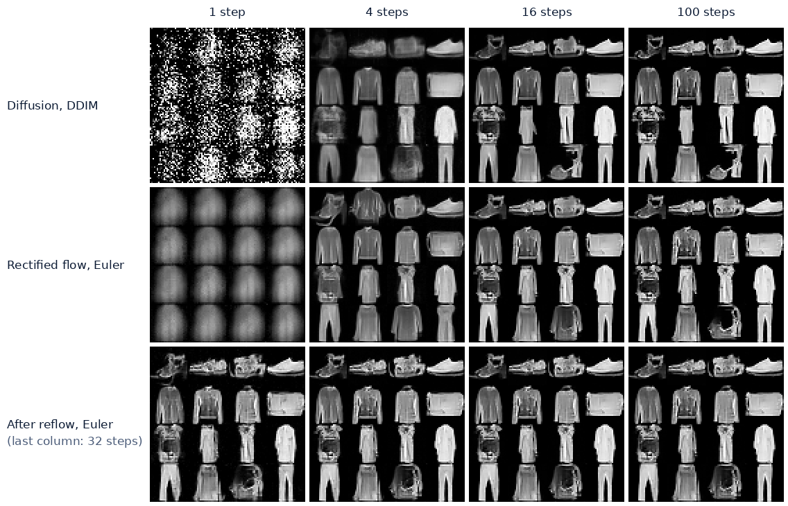
From 16 steps on, the diffusion model and the flow model mostly turn each noise image into the same garment. Trained separately with different objectives, they learned nearly the same map from noise to images and differ mainly in the steps they need.
Step 3: how straight are the paths?
A 2D picture
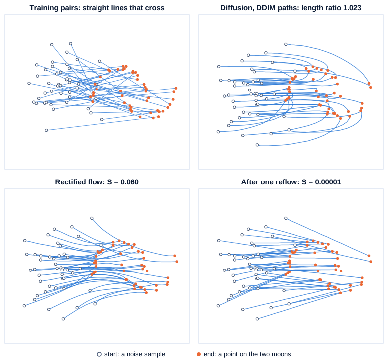
To see the paths, the same three methods were trained on a 2D toy problem: Gaussian noise to two interleaved half-moons. Three small MLPs (three hidden layers of 256), 12,000 steps of batch 1,024 each, ran on the CPU in under 3 minutes apiece. The reflow model was fine-tuned on 50,000 (noise, sample) pairs that the first flow produced with 200 Euler steps.
Swipe to pan the diagram, or tap it to zoom.
Flow matching trains on the first panel’s crossing lines and learns the third panel’s paths, which bend around each other because an ODE gives one velocity at each point. Reflow keeps the endpoints and removes the bends.
Liu et al.’s straightness S is the average squared gap between the velocity along a path and the straight-line velocity from its start to its end. Divided by the squared start-to-end distance, it falls from 0.060 for rectified flow to 0.00001 after reflow. The length ratio, a path’s length over the straight distance between its ends, is 1.023 for diffusion, 1.011 for rectified flow and 1.000002 after reflow. One-step samples tell the same story: their sliced Wasserstein distance to fresh data (the average gap between sorted 1D projections of two point clouds; 5 seeds of 5,000 points) is 2.72 for diffusion, 1.03 for rectified flow and 0.034 after reflow, the same as two samples of real data.
In 784 dimensions
The same diagnostics on Fashion-MNIST used 1,000 trajectories of 100 steps from each trained model. A length ratio of 1.0 means perfectly straight. S is left out for DDIM, whose steps are evenly spaced in noise level rather than in time, so its velocities aren’t on the same scale.
| Model and sampler | Length ratio, mean ± SD | Largest gap from the straight line, as a share of its length | S, normalized |
|---|---|---|---|
| Diffusion U-Net, DDIM | 1.113 ± 0.016 | 0.41 | not comparable |
| Flow U-Net, Euler | 1.025 ± 0.009 | 0.078 | 0.053 |
| Flow DiT, Euler | 1.028 ± 0.010 | 0.084 | 0.059 |
| Flow U-Net after reflow | 1.0014 ± 0.0006 | 0.017 | 0.0028 |
The diffusion paths come out 11.3% longer than their chords, almost exactly the quarter circle’s 11.1% from Step 1, so most of their bend comes from the noise schedule itself. Rectified flow paths are within 3% of straight, and reflow takes them to 0.14%, with S down 19 times. The DiT’s paths match the U-Net’s, since straightness depends on the training objective.
These numbers also explain the tie in Step 2. At its furthest, a rectified flow path sits on average 7.8% of its length away from the straight line, enough to ruin a 1-step sample. Reflow brings that to 1.7%.
Step 4: the denoiser becomes a transformer
Patchify, then a plain ViT
The Diffusion Transformer, DiT (Peebles and Xie, 2022), replaces the U-Net with the vision transformer from Part 2. The noisy latent is cut into p × p patches and each patch becomes one token. The tokens get fixed 2D sine-cosine position vectors, and a stack of transformer blocks predicts the noise for every patch. A final linear layer turns each token back into a p × p patch of output.
A 256-pixel image has a 32 × 32 × 4 latent (Part 1 measured the 512-pixel version), so 2 × 2 patches give 256 tokens. The tiny DiT trained here works on Fashion-MNIST pixels: 196 tokens of width 192 through 6 blocks with 6 heads, 4.16 million parameters.
adaLN-Zero: how the timestep gets in
A denoiser has to know how noisy its input is, and usually what to draw. LayerNorm (layer normalization, Math Part 10) rescales each token vector to zero mean and unit spread, then applies a learned scale and shift. In adaptive LayerNorm (adaLN), a small MLP computes that scale and shift from the timestep and label, so the same block behaves differently at each noise level. adaLN-Zero adds a gate on each sub-layer’s output, produced by a layer that starts at zero, so every block starts as the identity function.
In the DiT paper’s Table 4, after 400,000 steps at about 118.6 GFLOPs (billions of floating-point operations per forward pass), adaLN-Zero scored FID 19.47 without guidance, against 25.21 for plain adaLN, 26.14 for cross-attention (at 137.6 GFLOPs) and 35.24 for feeding the condition in as extra tokens.

Compute, not parameters
DiT’s 12 models, four sizes times three patch sizes (8, 4, 2), show “a strong negative correlation between model Gflops and FID-50K” (−0.93). Smaller patches barely change the parameter count but multiply the tokens, and quality follows the compute: DiT-XL/8 and DiT-XL/2 both have about 675 million parameters, but at 7.39 against 118.64 GFLOPs they scored FID 106.41 against 19.47.
Sampling longer did not make up for a smaller model: DiT-XL/2 at 128 steps used 5 times less compute per image than DiT-L/2 at 1,000 steps and still scored better (FID-10K 23.7 against 25.9). Trained longer and sampled with guidance, DiT-XL/2 reached FID 2.27 on class-conditional ImageNet at 256 × 256, beating latent diffusion’s 3.60 (all reported by Peebles and Xie, not reproduced here).
A tiny DiT against a tiny U-Net
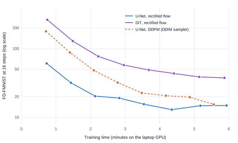
The 4.16M-parameter DiT was trained with the rectified flow objective and the U-Nets’ recipe, and EMA snapshots every 500 steps were scored on 2,000 samples at 16 steps, with the same noise each time.
Swipe to pan the diagram, or tap it to zoom.
| Measure | U-Net | DiT |
|---|---|---|
| Parameters | 4.10M | 4.16M |
| Forward pass, per image | 1.03 GFLOPs | 1.22 GFLOPs |
| Training, images per second (batch 128) | 1,561 | 1,447 |
| Sampling throughput, image-steps per second (batch 1,000) | 3,629 | 4,167 |
| One network call for one image | 9.2 ms | 4.4 ms |
| FD-FMNIST after 4,000 steps (16 steps) | 14.9 | 37.7 |
Throughput is the median of 7 timed bf16 runs after warm-up, with torch.cuda.synchronize() around each. The DiT does 19% more arithmetic per image yet samples faster, because its work is a few large matrix multiplies while the U-Net runs many small convolutions and normalizations.
Quality goes the other way. After 352 seconds of training the DiT reached 37.7, a score the U-Net had passed between its 500th and 1,000th step, 44 to 86 seconds in. This is Part 2’s result again: at a few million parameters and a few minutes of training, a convolutional network’s built-in locality beats a transformer that has to learn it. DiT’s case rests on the scaling curve from 0.36 to 118.6 GFLOPs over hundreds of thousands of steps, and a laptop shows only its starting point.
The chart also shows the flow U-Net learning faster than the DDPM U-Net (FD 32 against 88 after 1,000 steps) until they meet at the end of training. That fits Lipman et al.’s report of “faster training” with straight paths, though here it rests on one run of each.
In the real world
- Stable Diffusion 3 (Esser et al., 2024) is a rectified flow model with logit-normal timesteps and an MM-DiT (multimodal diffusion transformer) backbone, in which text and image tokens get “two separate sets of weights” but attend to each other in one sequence. Text comes from three frozen encoders: CLIP-L/14 and CLIP-G/14 (77 tokens each; see Part 3) and the 4.7-billion-parameter T5-XXL. The largest model has 8 billion parameters, and its 16-channel latent reconstructs at FID 1.06 against 2.41 for 4 channels.
- Stable Diffusion 3.5 Large (model card) is an 8-billion-parameter MMDiT “that use[s] three fixed, pretrained text encoders, and with QK-normalization to improve training stability”. Downloads are gated under the Stability Community License, free for organizations under $1M in annual revenue.
- FLUX.1 [schnell] (model card) is “a 12 billion parameter rectified flow transformer” under Apache-2.0, “trained using latent adversarial diffusion distillation” to generate “in only 1 to 4 steps”. Its example runs 4 steps with guidance 0. FLUX.1 [dev] (model card), also 12 billion parameters, is “trained using guidance distillation” and released under a non-commercial license. Its example runs 50 steps at guidance 3.5.
- None of these fit the laptop used here: T5-XXL alone needs 9.4 GB in 16-bit precision, more than the GPU’s 8 GB.
- Distillation, training a fast student to copy a slow teacher, goes further than straight paths. Progressive distillation (Salimans and Ho, 2022) halves the step count repeatedly, reaching FID 3.0 on CIFAR-10 in 4 steps. Consistency models (Song et al., 2023) map any point on an ODE path directly to its end. LADD adds a discriminator and turned SD3’s 8B model into SD3-Turbo at “only four unguided sampling steps”. InstaFlow (Liu et al., 2023) reflowed Stable Diffusion and distilled it to one step: FID 13.1 on MS COCO 2014-30k in 0.09 seconds. All reported by their authors, not reproduced here.
Common misconceptions
- “Flow matching needs fewer steps than diffusion.” Not by itself. Trained with the same network and compute, rectified flow with Euler steps and DDPM with DDIM steps scored within their seed ranges of each other from 4 to 100 steps. The few-step gains come from straightening the learned paths (reflow) or from distillation.
- “Training on straight lines gives straight paths.” The training lines cross, and the network can only learn their average at each point, so the learned paths bend. In 2D the straightness measure went from 0.060 to 0.00001 only after reflow.
- “Flow matching and diffusion are different kinds of model.” Both mix image and noise,
a × image + b × noise, and learn to undo it. They differ in the path (quarter circle or straight line) and the target (noise or velocity), and DDIM is itself an Euler solver for an ODE. - “Transformers beat U-Nets at image generation.” At equal size and a few minutes of training, the U-Net won clearly here: FD 14.9 against 37.7. DiT’s advantage is that quality keeps improving as compute grows, from FID 106 to 19 at the same 675 million parameters in the DiT paper.
Key takeaways
- Flow matching trains a network to predict one velocity, image minus noise, along a straight line, and sampling follows it with Euler steps.
- Straight training lines don’t make straight learned paths. Without reflow, rectified flow matched diffusion with DDIM step for step on Fashion-MNIST: about 130 at 4 steps and 9 at 32.
- One round of reflow straightened the paths: the length ratio fell from 1.025 to 1.0014, and the one-step score improved from 724 to 46.5, at some cost at high step counts.
- Diffusion’s paths are about 11% longer than straight lines, the quarter-circle geometry of its noise schedule.
- A DiT is a ViT over latent patches, conditioned through adaLN-Zero gates. It scales with compute, but at 4 million parameters a U-Net beat it by more than two to one.
What’s next
Diffusion and flow models both refine all of an image’s pixels at once. Part 8 takes the other road: it turns the image into a sequence of discrete tokens and generates it the way a language model writes text, one token at a time or many at once, then lets one transformer both read and write images.
Further reading
- Scalable Diffusion Models with Transformers (Peebles and Xie, 2022): DiT; patchified latents, adaLN-Zero, and the Gflops-versus-FID scaling result.
- Flow Straight and Fast: Learning to Generate and Transfer Data with Rectified Flow (Liu et al., 2022): rectified flow, the straightness measure, reflow and one-step distillation.
- Flow Matching for Generative Modeling (Lipman et al., 2022): conditional flow matching, Gaussian probability paths, and the optimal transport path compared with diffusion paths.
- Scaling Rectified Flow Transformers for High-Resolution Image Synthesis (Esser et al., 2024): Stable Diffusion 3; 61 formulations compared, logit-normal timesteps, MM-DiT and the 16-channel latent.
- Denoising Diffusion Implicit Models (Song et al., 2020): the deterministic DDIM sampler used for the diffusion baseline, and its reading as an Euler solver.
- Denoising Diffusion Probabilistic Models (Ho et al., 2020): the noise-prediction objective and linear schedule used for the baseline.
- Progressive Distillation for Fast Sampling of Diffusion Models (Salimans and Ho, 2022), Consistency Models (Song et al., 2023), Adversarial Diffusion Distillation (Sauer et al., 2023) and Fast High-Resolution Image Synthesis with Latent Adversarial Diffusion Distillation (Sauer et al., 2024): four routes to few-step samplers.
- InstaFlow: One Step is Enough for High-Quality Diffusion-Based Text-to-Image Generation (Liu et al., 2023): reflow and distillation applied to Stable Diffusion.
- Model cards: Stable Diffusion 3.5 Large, FLUX.1 [schnell] and FLUX.1 [dev].
- Fashion-MNIST (Xiao et al., 2017): the clothing images used for every image experiment here (MIT license, Zalando Research).