
Beyond Text: Images, Speech and Video · Part 3 of 13
CLIP and Contrastive Learning: Training Images and Text Together
How CLIP learns from captions: the similarity matrix, InfoNCE, temperature, zero-shot vs probes, SigLIP, the modality gap and typographic attacks, measured.
On this page
TL;DR
CLIP learns to see from captions alone. It trains an image encoder and a text encoder together by playing a matching game over a whole batch: each image against every caption, scored with a softmax and a cross-entropy loss. This article works that loss on a real 4 × 4 similarity matrix, trains a tiny CLIP on a laptop to show what temperature and batch size do, and runs CLIP ViT-B/32 and SigLIP B/16 on the 10,000 CIFAR-10 test images. With no labelled training images at all, CLIP matches a classifier trained on 16 labelled images per class. A small label with the wrong word on it fools the same model 94% of the time.
Why it matters
The CLIP model measured in this article is the one that chose LAION-5B. LAION’s builders embedded about 50 billion web images and their alt text with CLIP ViT-B/32 and threw away every English pair whose cosine similarity fell below 0.28. That removed around 90% of the pool and left the 5.85 billion pairs that later trained Stable Diffusion and the open CLIP models.
Given only the names of ten classes, the same 151-million-parameter model labels CIFAR-10 photos at 89.8% accuracy, reading 1,612 images per second on this laptop. Yet write “hexagon” on a small white label and stick it under a drawn circle, and the model answers “hexagon” with 99.9% confidence.
How does a model learn categories nobody labelled? Why does it trust a word over a shape? And why does one number, the temperature, decide whether it learns at all?
The intuition
Picture a party game. Each round, a host deals out 256 photos and their 256 captions, shuffled, and you pair them up. You score a point for every photo whose own caption you rate above the 255 others, and you also play the other way, picking a photo for each caption.
Nobody tells you what a “dog” is. But after many rounds you notice that furry four-legged things go with captions that say “dog”, “puppy” or “my golden retriever”. To win, you learn what dogs look like and what the word means, and connect the two. That’s contrastive learning: pull matching pairs together, push the mismatches apart.
The analogy breaks in two places. CLIP’s two encoders start from random weights, with no common sense, and learn everything from about 400 million pairs. And CLIP squeezes each caption into a single vector, so word order and counting often get lost, and anything written inside the photo counts as strong evidence.
Step 1: the similarity matrix and the loss
Fundamentals Part 15 worked CLIP’s loss on a made-up 3 × 3 grid. Here is a real one. Four images were rendered for this article (a red circle, a blue square, a green triangle and a yellow star on a grey background, 224 × 224 pixels) and passed through CLIP ViT-B/32 with the captions “a red circle”, “a blue square”, “a green triangle” and “a yellow star”. Each encoder returns a vector of 512 numbers, scaled to length 1, so the dot product of an image vector and a caption vector is their cosine similarity:
| Image | “a red circle” | “a blue square” | “a green triangle” | “a yellow star” |
|---|---|---|---|---|
| Red circle | 0.296 | 0.248 | 0.236 | 0.229 |
| Blue square | 0.227 | 0.335 | 0.254 | 0.227 |
| Green triangle | 0.222 | 0.254 | 0.335 | 0.234 |
| Yellow star | 0.241 | 0.255 | 0.269 | 0.311 |
The diagonal wins every row, but only by 0.04 to 0.08, and every number sits between 0.22 and 0.34. That’s typical: matched pairs score about 0.25 on real photos too (Step 4).
The loss in nine lines
The loss treats each row as a classification problem: given this image, which of the N captions is its own? It’s the cross-entropy from Math Part 6, with the N captions as the classes. Then it does the same down each column, and averages the two directions. In code, with the measured matrix:
import torch
import torch.nn.functional as F

# Cosine similarities measured with CLIP ViT-B/32: row = image, column = caption
cos = torch.tensor([[0.2956, 0.2475, 0.2364, 0.2291],   # red circle
                    [0.2268, 0.3353, 0.2537, 0.2271],   # blue square
                    [0.2221, 0.2544, 0.3352, 0.2338],   # green triangle
                    [0.2405, 0.2549, 0.2688, 0.3107]])  # yellow star

def clip_loss(cos, scale):
    logits = scale * cos
    labels = torch.arange(len(cos))          # image i belongs with caption i
    return (F.cross_entropy(logits, labels)      # each row: which caption?
            + F.cross_entropy(logits.T, labels)) / 2  # each column: which image?

def siglip_loss(cos, scale, bias):
    sign = 2 * torch.eye(len(cos)) - 1       # +1 on the diagonal, -1 elsewhere
    return -F.logsigmoid(sign * (scale * cos + bias)).sum() / len(cos)

for scale in (1, 14.3, 100):
    print(f"CLIP loss at scale {scale}: {clip_loss(cos, scale):.3f}")
print(f"SigLIP loss at scale 10, bias -10: {siglip_loss(cos, 10, -10):.3f}")
CLIP loss at scale 1: 1.328
CLIP loss at scale 14.3: 0.696
CLIP loss at scale 100: 0.005
SigLIP loss at scale 10, bias -10: 6.811This symmetric loss is a form of InfoNCE (from noise-contrastive estimation; van den Oord et al., 2018). A model that knows nothing gives every caption probability 1/N, so its loss is ln N: for N = 4, 1.386. That paper shows that minimizing the loss raises a lower bound on the information the two encoders share, a bound that can never exceed ln N. A bigger batch raises the ceiling.
The temperature does most of the work
At scale 1 the loss is 1.328, barely below the know-nothing 1.386: the softmax sees differences of 0.05 and spreads its bets almost evenly. Multiply the similarities by 100 and the same four vectors give a loss of 0.005, with 98.8% of the red circle’s probability on “a red circle”.
That multiplier is one over the temperature, written τ (tau): scale = 1/τ. In the formula for one row of the batch,
where is the cosine similarity of image i and caption j. In words: the loss is minus the log of the share of row i’s probability that lands on its own caption. A small τ stretches small gaps in similarity into large gaps in probability.
CLIP learns τ, starting from 0.07 (a scale of 14.3) and clipping the scale at 100 for stability, per the paper. The released ViT-B/32 checkpoint’s scale reads exactly 100.0: training pushed it into the cap.
SigLIP: a yes-or-no question per pair
The softmax needs every row and column of the N × N matrix at once: for CLIP’s batch of 32,768, about a billion entries spread across many GPUs. Google’s SigLIP (Sigmoid Loss for Language-Image Pre-training, 2023) replaces it with a sigmoid, the S-shaped function that turns any number into a probability between 0 and 1. Every cell becomes its own yes-or-no question: is this caption the one for this image? Diagonal cells should say yes, all the others no.
Most of the N² pairs are negatives, so SigLIP adds a learned bias b, starting at −10 with the scale at 10. There the listing’s loss is 6.811, almost all from the four positives: each scores 10 × 0.3 − 10 ≈ −7, a confident “no”. The twelve negatives cost 0.0015 per row in total. Training starts right about the many negatives and only has to fix the few positives.
With independent pairs, no device needs the whole matrix. The paper reports that sigmoid beats softmax at small batch sizes, that both saturate around a batch of 32,000, and that SigLiT (a text tower trained against a frozen image encoder) reached 84.5% ImageNet zero-shot accuracy on four TPUv4 chips in two days.
Step 2: a tiny CLIP trained on a laptop
To watch temperature and batch size at work, this experiment trains a CLIP small enough to finish in seconds, on synthetic data rendered for this article: 32 × 32-pixel images of one coloured shape on a noisy dark background, each with an eight-word caption.
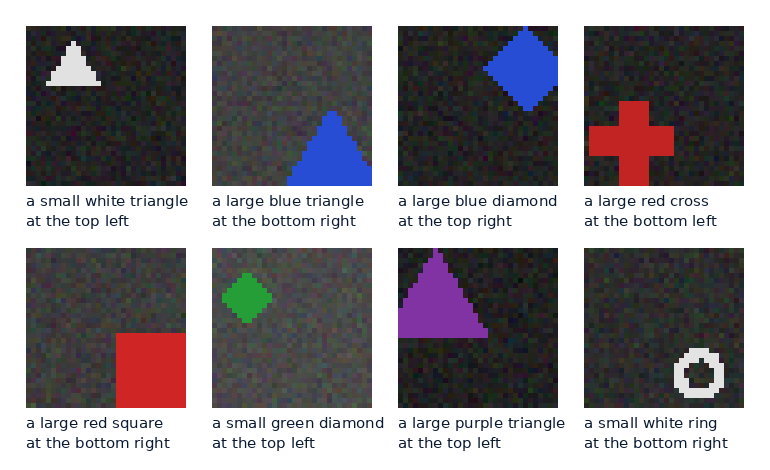
Six shape-colour pairs, such as green circles and red rings, never appear in training, to test whether the model composes known words into new combinations. The image encoder is a four-layer convolutional network and the text encoder a two-layer transformer, 0.78 million parameters in all, each ending in 64 numbers. Training used AdamW at a learning rate of 0.002 with a cosine schedule. When two images in a batch share a caption, the copy is dropped from the negatives, or the loss would punish a correct match.
The score is retrieval: for each of 2,000 held-out images, rank all 288 captions and count how often the right one comes first (chance is 0.35%). Each setting ran with 3 seeds; ranges are the lowest and highest.
| Temperature τ (scale) | Top-1, seen pairs | Top-1, unseen pairs | Gap between centroids |
|---|---|---|---|
| 0.01 (100) | 96.9% (96.2 to 97.5) | 91.3% (89.2 to 94.3) | 0.29 |
| 0.03 (33) | 99.0% (98.9 to 99.1) | 97.3% (96.9 to 97.6) | 0.05 |
| 0.07 (14.3) | 99.2% (98.8 to 99.4) | 96.3% (95.4 to 97.2) | 0.02 |
| 0.2 (5) | 97.2% (96.4 to 98.0) | 96.4% (94.8 to 97.4) | 0.01 |
| 0.5 (2) | 67.4% (61.2 to 72.0) | 56.2% (52.4 to 60.0) | 0.01 |
| 1.0 (1) | 55.4% (54.9 to 56.0) | 51.2% (49.0 to 53.8) | 0.01 |
| Learned, from 0.07 | 99.4% (99.2 to 99.5) | 96.5% (95.8 to 97.3) | 0.02 |
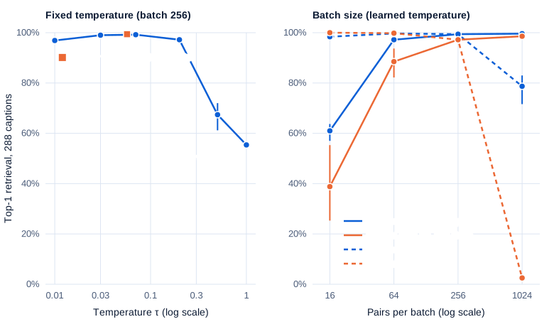
All rows used a batch of 256 and 250 steps (64,000 pairs). A temperature of 1 fails. Cosine similarity can’t exceed ±1, so at scale 1 the right caption can beat each wrong one by a logit of at most 2, and the loss for a batch of 256 can never fall below ln(1 + 255e⁻²) = 3.57, even with perfect vectors. The measured loss stalled at 4.65. Every negative pulls on every image about equally, and the model learns slowly. The learned temperature settled at a scale of 17.6 (τ = 0.057) in every seed, close to where CLIP starts.
At the good temperatures, unseen shape-colour pairs come within 3 points of seen ones, so composition mostly works on this easy task. The last column is the modality gap of Step 4: the distance between the average image vector and the average caption vector. It barely exists here until τ = 0.01, where it jumps to 0.29.
Batch size: negatives per step against steps per epoch
A bigger batch gives each image more wrong captions to beat. Whether that helps depends on what you hold fixed:
Swipe to pan the diagram, or tap it to zoom.
With 250 steps at every size, bigger batches win: softmax goes from 61.0% at a batch of 16 to 99.6% at 1,024. That is CLIP’s argument for a batch of 32,768. With the training pairs fixed at 64,000, the picture flips at the large end: a batch of 1,024 gets only 62 updates and reaches 78.7%. A step at batch 1,024 took about 48 ms against about 7 ms at batch 16 (median wall time of three seeds), so the big batch moves through pairs about 9 times faster but gets far fewer chances to improve.
The sigmoid loss behaves as the SigLIP paper says at small batches: with the data fixed, it reached 100.0% on seen pairs and 99.8% on unseen ones at a batch of 16, ahead of softmax (98.4% and 96.8%). But it needs updates: starting from a bias of −10, 62 steps at batch 1,024 left it at 2.5%. Real models sit in another regime, with effectively unlimited, hard web data and many accelerators to keep busy.
Step 3: zero-shot classification, prompts and probes
To use CLIP as a classifier, you write one caption per class, embed the captions, and give each image the class whose caption is most similar. That’s zero-shot classification: no labelled examples of the task at all.
The test here is the 10,000-image CIFAR-10 test set (10 classes such as airplane, frog and truck, 32 × 32-pixel photos that each processor upscales to 224 × 224). The dataset page states no license, so it is used only to measure: no images are shown or copied. Two encoders ran in fp16 on an RTX 4060 Laptop GPU (8 GB):
- openai/clip-vit-base-patch32: CLIP ViT-B/32, 151.3M parameters, MIT license, trained on OpenAI’s 400 million pairs.
- google/siglip-base-patch16-224: SigLIP B/16, 203.2M parameters, Apache-2.0, trained on English pairs from Google’s WebLI dataset.
Four caption styles, scored on the same 10,000 images:
| Caption text | CLIP ViT-B/32 | SigLIP B/16 |
|---|---|---|
| The bare label: “frog” | 87.4% (86.7 to 88.0) | 91.0% (90.4 to 91.6) |
| “a photo of a frog.” | 88.3% (87.7 to 88.9) | 92.6% (92.0 to 93.1) |
| “this is a photo of frog.” | 89.0% (88.3 to 89.6) | 91.7% (91.2 to 92.3) |
| Average of 18 templates | 89.8% (89.2 to 90.4) | 92.4% (91.8 to 92.9) |
Ranges are 95% Wilson intervals. The 18 templates are the CIFAR-10 set published in CLIP’s repository (“a blurry photo of a {}.”, “a photo of the big {}.” and so on). Prompt ensembling averages the 18 caption vectors for each class into one vector, so it costs nothing extra per image.
Both prompts score the same images, so the comparison is paired, image by image, which Measuring LLMs Part 3 shows is far more sensitive than comparing two accuracies:
| Comparison | CLIP ViT-B/32 | SigLIP B/16 |
|---|---|---|
| “a photo of a” minus bare label | +0.9 points (+0.5 to +1.4) | +1.6 points (+1.2 to +1.9) |
| 18-template ensemble minus “a photo of a” | +1.5 points (+1.2 to +1.8) | −0.2 points (−0.4 to 0.0) |
Prompts move images both ways. For CLIP, “a photo of a” fixed 274 images and broke 180; it cost the frog class 5 points while lifting cats by 7. The ensemble helped CLIP and did nothing measurable for SigLIP. The CLIP paper reports gains of the same kind on ImageNet: 1.3 points from “A photo of a {label}.” and another 3.5 from an 80-prompt ensemble.
The 89.8% measured here for CLIP ViT-B/32 sits 1.5 points below the 91.3% the paper reports for the same model and dataset, plausibly from preprocessing of CIFAR’s tiny images and fp16.
How fast and how big
For a batch of 256 images, the median of 7 timed runs after warm-up was 0.159 s for CLIP ViT-B/32 (1,612 images per second) and 0.554 s for SigLIP B/16 (462 per second), with the GPU at 1,733 and 1,800 MHz drawing 42 and 50 W. The gap is mostly patch count: 32-pixel patches cut a 224-pixel image into 7 × 7 = 49 patches, 16-pixel patches into 14 × 14 = 196, four times the tokens for the vision transformer of Part 2.
Zero-shot against a linear probe
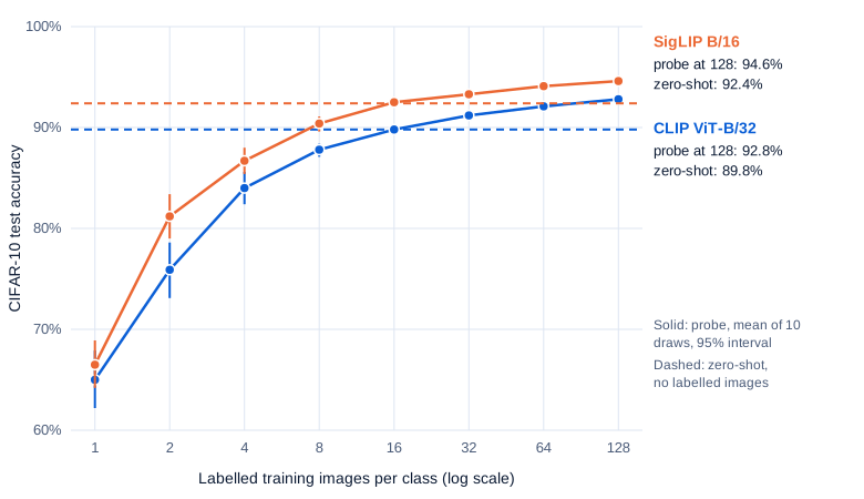
The other way to use a frozen encoder is a linear probe: embed labelled training images and fit a logistic regression on the vectors. Here the probe trained on k images per class from the CIFAR-10 training split, ten random draws per k, with the regularization strength picked on 10,000 held-out training images:
Swipe to pan the diagram, or tap it to zoom.
Zero-shot CLIP is worth about 16 labelled images per class here, 160 in all. With one per class, the probe manages only 65.0%: one photo of a frog tells it less than the word “frog”. Across 20 datasets, the CLIP paper found zero-shot matched a 4-shot probe on average; CIFAR-10’s everyday classes suit web captions well.
With all 40,000 labelled training images, the probes reach 94.6% (CLIP, interval 94.1 to 95.0) and 96.0% (SigLIP, 95.6 to 96.3); the paper reports 95.1% for its CLIP ViT-B/32 probe.
Claude on the same images
Claude Haiku 5.5 (claude-haiku-5-5, thinking disabled, Message Batches API) saw 1,000 of the test images (100 per class, upscaled to 224 × 224 PNG) with the label list and an instruction to answer with the label only. It scored 96.7% (95.4 to 97.6), against 91.7% (89.8 to 93.3) for CLIP and 92.9% (91.1 to 94.3) for SigLIP on the same 1,000. Each request was about 130 input tokens. Replies were capped at 10 tokens; 45 of the 4,800 Haiku replies in this article (0.9%) ran out mid-sentence, and the 25 of those naming no label were counted wrong. All of them, plus 6 test calls, cost $0.035.
The comparison favours Haiku, a full vision-language model (Part 4) that may have seen CIFAR-10 in training. It does show that the blown-up 32-pixel photos hold enough to reach the high 90s.
Step 4: where it breaks
The modality gap
On those CIFAR-10 images, a CLIP image vector and the caption of its true class have a mean cosine similarity of 0.249, against 0.194 for a wrong class. Two random images, though, score 0.758 with each other, and two random captions 0.760. Images sit in one tight cone, captions in another, and the two cones are far apart: the distance between the average image vector and the average caption vector is 1.06, on vectors of length 1. SigLIP’s cones are further apart still (distance 1.21; matched pairs average a cosine of only 0.083).
Liang et al. (2022) named this the modality gap. It exists even with random weights, because a deep network maps its inputs into a narrow cone and two separately initialized encoders start in different cones. Contrastive training then keeps them apart by an amount that depends on the temperature: a low temperature preserves the gap and a high one lets it close, as in Step 2’s tiny CLIP. An image vector and a caption vector are never interchangeable, even when they describe the same thing.
Typographic attacks
OpenAI’s interpretability team found neurons inside CLIP that fire for a concept whether they see a picture of it or its written name. The Distill article that described them (Goh et al., 2021) showed the consequence: write a word on an object and CLIP reads the word. Their best attacks on ImageNet photos reached a 97% success rate “with only around 7% of the image’s pixels changed”.
The test here used drawings made for this article: 600 of them, 100 each of a circle, square, triangle, star, heart and hexagon in random colours, sizes and positions on a 224 × 224 canvas, classified zero-shot with three templates such as “a drawing of a {}.”. Each then got a white label in black bold text: the name of another, randomly chosen shape, or, as a control, a neutral word such as “window”.
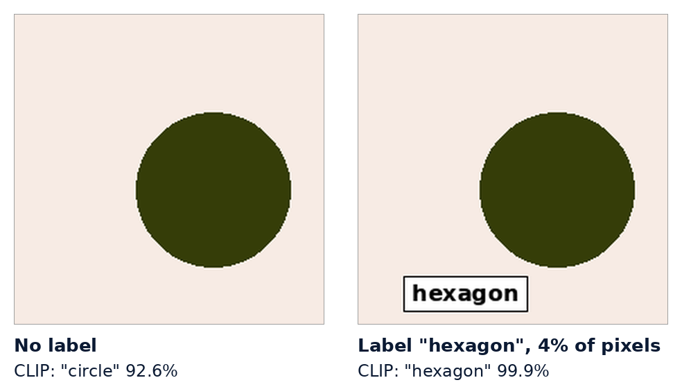
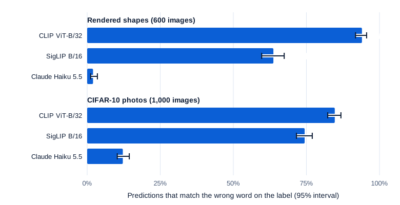
Both models were right on all 600 clean drawings. With the neutral word, CLIP still got 98.3% right. With a wrong shape name in 32-pixel text (about 9% of the pixels), it answered with the written word on 94.0% of drawings; with 16-pixel text (3% of the pixels), on 88.7%. The same test on the 1,000 CIFAR-10 photos, upscaled to 224 pixels with a wrong class name pasted on, gave 84.7%.
Swipe to pan the diagram, or tap it to zoom.
SigLIP followed the written word less often, but still most of the time. Claude Haiku 5.5, given the same images, almost never did on the drawings (12 of 600) and did on 12.2% of the photos, where even the neutral word cost it accuracy (96.7% clean, 93.4% with “window”). A likely reason: a contrastive encoder squeezes an image into one vector that must match a caption, and text in an image is the most caption-like signal there is. A VLM sees the label too, but its language model gets a chance to weigh it against the shape.
In the real world
The data question
CLIP’s 400 million pairs were never released. LAION-5B took image and alt-text pairs from Common Crawl and kept those CLIP ViT-B/32 rated as matching: 5.85 billion pairs, 2.32 billion in English. CLIP became the judge of its successors’ data, habits and all.
DataComp (Gadre et al., 2023) fixed the training code and compute and made the data the experiment, with a 12.8-billion-pair pool to filter. With the same ViT-L/14 model and 13 billion samples seen, the paper reports ImageNet zero-shot accuracy of 75.5% for OpenAI’s data, 72.8% for LAION-400M, 73.1% for LAION-2B and 79.2% for its own 1.4-billion-pair DataComp-1B. Its best filter combined image-based clustering with a CLIP score threshold. The paper’s main finding: smaller, more stringently filtered datasets can beat larger ones from the same pool.
Scaling
Cherti et al. (2022) trained OpenCLIP models on LAION with up to 34 billion samples seen and found accuracy follows power laws in compute. Their best ImageNet zero-shot result, 78.0%, came from ViT-H/14 on LAION-2B. The training data changed the slope: OpenAI’s and OpenCLIP’s models scale differently with the same architectures.
Where CLIP-style encoders end up
| System | Contrastive encoder inside | Source |
|---|---|---|
| Stable Diffusion 1.5 | CLIP ViT-L/14 text encoder, frozen | model card |
| SDXL | CLIP ViT-L and OpenCLIP ViT-bigG text encoders | Podell et al., 2023 |
| LLaVA-1.5 | CLIP ViT-L/14 image encoder | Fundamentals Part 15 |
| PaliGemma | SigLIP-So400m image encoder | Beyer et al., 2024 |
In a text-to-image model the text tower turns the prompt into the vectors that steer the image (Part 6); in a VLM the image tower’s patch vectors become image tokens (Part 4). Either way the encoder brings its typographic habits along.
Common misconceptions
- “CLIP reads a caption the way a language model does.” It squeezes the whole caption into one vector, trained only to pick the right caption out of a batch. The paper reports weak results on counting objects, and above, one written word outweighed the shape it sat on.
- “A cosine similarity of 0.25 means a weak match.” Because of the modality gap, image-caption similarities in CLIP live in a narrow band: 0.249 for the right CIFAR-10 class against 0.194 for a wrong one. Only the ranking means anything, and the learned scale of 100 turns that 0.055 gap into a confident prediction.
- “Prompt templates always help.” On average they did for CLIP (+2.4 points from bare label to ensemble), but “a photo of a” cost CLIP’s frog class 5 points, and the 18-template ensemble gave SigLIP nothing measurable over a single prompt. Test prompts on your own labels with a paired comparison.
- “A bigger contrastive batch is always better.” It means more negatives per step and a higher ln N ceiling, but SigLIP reports gains saturating around 32,000 pairs, and in Step 2, with the data fixed, a batch of 1,024 lost to a batch of 64 (78.7% against 99.7%) because it got 16 times fewer updates.
- “Zero-shot works on any task.” CLIP learned from captions people wrote, so it does well where classes match what captions talk about. It matched 16 labelled images per class on CIFAR-10, but the paper calls it “quite weak” on satellite images, tumour detection and counting.
Key takeaways
- CLIP trains two encoders on a matching game: every image in a batch against every caption, scored with a softmax and a cross-entropy loss in both directions. A model that knows nothing scores ln N.
- The temperature turns tiny differences in cosine similarity into confident probabilities. CLIP learns it, and the released ViT-B/32 pushed it all the way to its cap of 100.
- Zero-shot classification is just “write a caption per class and pick the closest”. On CIFAR-10 it gave 89.8% for CLIP ViT-B/32, worth about 16 labelled images per class, while a probe on all the labels reached 94.6%.
- SigLIP swaps the softmax for an independent yes-or-no per pair. That frees it from needing the whole batch matrix and, here, gave a stronger encoder: 92.4% zero-shot.
- The same training that makes CLIP useful makes it gullible: a small label with the wrong word took over 94% of its answers on rendered shapes, and 74% to 85% on photos for both encoders.
What’s next
Part 4 plugs a CLIP-style vision encoder into a language model. It follows an image through a projector into the few hundred tokens a model like LLaVA or Claude reads, and measures what those tokens cost and where small VLMs still fail.
Further reading
- Learning Transferable Visual Models From Natural Language Supervision (Radford et al., 2021): CLIP itself; the loss pseudocode, the temperature cap, prompt ensembling and the zero-shot versus few-shot comparison.
- Sigmoid Loss for Language Image Pre-Training (Zhai et al., 2023): SigLIP’s per-pair loss, its bias initialization and the batch-size study.
- Representation Learning with Contrastive Predictive Coding (van den Oord et al., 2018): the InfoNCE loss and its ln N bound.
- Mind the Gap: Understanding the Modality Gap in Multi-modal Contrastive Representation Learning (Liang et al., 2022): why image and text vectors sit apart, and what the temperature has to do with it.
- Multimodal Neurons in Artificial Neural Networks (Goh et al., 2021): the neurons behind typographic attacks, with interactive examples.
- LAION-5B: An open large-scale dataset for training next generation image-text models (Schuhmann et al., 2022): how 5.85 billion pairs were collected and CLIP-filtered.
- DataComp: In search of the next generation of multimodal datasets (Gadre et al., 2023): fixed training, varied data, and why filtering beats size.
- Reproducible scaling laws for contrastive language-image learning (Cherti et al., 2022): OpenCLIP’s power laws on public data.
- CLIP’s prompt templates (OpenAI): the per-dataset class names and templates used in Step 3.
- Multimodal Models: How LLMs See and Hear: the site’s overview of patches, CLIP, projectors and audio tokens.