
Beyond Text: Images, Speech and Video · Part 4 of 13
Vision-Language Models: How an Image Becomes Tokens
Projectors, Q-Formers and cross-attention, tiling and pixel shuffle, what an image costs, and five checkable tasks run on SmolVLM, Qwen2-VL and Claude.
On this page
TL;DR
A vision-language model (VLM) is a vision encoder, a language model and a small connector that turns the encoder’s output into something the language model can read. This article compares the three classic connectors (LLaVA’s projector, BLIP-2’s Q-Former and Flamingo’s cross-attention), the ways they take in large images, and how they’re trained. Then it measures what an image costs in tokens and time, and runs five checkable tasks on two small open VLMs and two Claude models at several image sizes, 100 items per condition. Image size decided whether small text could be read at all, and Claude Haiku 5.5 counted accurately only when it counted out loud.
Why it matters
Claude Haiku 5.5 read a five-character code off an 896-pixel image 100 times out of 100. Shrink the same image to 224 pixels, where the type is 3 to 8.5 pixels in size, and it got 43 right; at 448 pixels, 74. Same model, same question, fewer pixels behind each token.
Cost moves just as fast. On Claude, a 224-pixel image is 67 tokens and a 1,792-pixel image 4,099. On SmolVLM-256M’s default settings both become 1,088 tokens, because the processor enlarges the small one before tiling it.
So what does a connector do with an image? Why can one model count 40 dots perfectly while another misses by 20? And when you pay for 4,000 image tokens, what are you buying?
The intuition
Think of a travel adapter. Your charger (the vision encoder) was built for one socket and the wall (the language model) has another; a small part in between makes them fit.
There are three common designs for that part. The simplest converts every pin one to one: each patch vector from the encoder becomes one token in the language model’s input. The second puts a summarizer in between: 32 learned “questions” read the whole image and pass on only their 32 answers. The third leaves the input alone and adds side doors on some floors of the building, so text can consult the image at those layers.
The analogy breaks in one place: an adapter is passive wiring, while the connector is trained on millions of image-text pairs to produce vectors the language model can use. Those vectors needn’t resemble any word in the vocabulary.
Step 1: three ways to connect a vision encoder
Fundamentals Part 15 introduced LLaVA’s projector and Flamingo’s cross-attention. Here they are next to BLIP-2’s Q-Former, with the numbers that set them apart.

Swipe to pan the diagram, or tap it to zoom.
The projector: one token per patch
LLaVA-1.5’s connector (Liu et al., 2023) is a two-layer MLP (multilayer perceptron: two matrix multiplications with a nonlinearity between them). CLIP ViT-L/14 at 336 pixels outputs 576 patch vectors of 1,024 numbers, and the MLP maps each to the 4,096 numbers of a Vicuna-7B embedding. That’s 1,024 × 4,096 + 4,096 × 4,096, about 21 million weights against 7 billion in the language model, and it’s the only part trained in the first stage. Every patch arrives as its own token, so detail survives, and so does the cost: 576 tokens for a blank wall or a page of text.
The Q-Former: a fixed-size summary
BLIP-2 (Li et al., 2023) puts a small Transformer, the Querying Transformer or Q-Former, between a frozen image encoder and a frozen language model. It starts from BERT-base weights, has 188 million parameters and owns 32 learned query vectors of 768 numbers. The queries read the image through cross-attention layers in every other block. (Cross-attention lets one set of vectors look up information in another.)
The output is always 32 × 768, against 257 × 1,024 for the ViT-L/14 features it reads. The paper calls this an information bottleneck that makes the queries keep the visual information “most relevant to the text.” One linear layer maps the 32 vectors to the language model’s width, in front of the text. BLIP-2 beat Flamingo-80B by 8.7 points on zero-shot VQAv2 (65.0 against 56.3) “with 54x fewer trainable parameters.” Thirty-two vectors are a small budget for a dense document, though.
Cross-attention: side doors into a frozen model
Flamingo (Alayrac et al., 2022) keeps the image out of the input sequence. Its Perceiver Resampler turns a variable number of encoder features into a fixed 64, using learned queries much like the Q-Former’s, and new gated cross-attention layers between the frozen language model’s blocks read them. Each text token attends only to the image just before it, which let Flamingo use up to 32 example pairs in a prompt after training on at most 5 images per sequence. The image takes up no context positions at all.
| Connector | Vectors per image | Where they enter | Trained in the first stage |
|---|---|---|---|
| Projector (LLaVA-1.5) | 576, one per patch | Input sequence | The MLP alone |
| Q-Former (BLIP-2) | 32 | Input sequence, before the text | The Q-Former alone |
| Resampler and cross-attention (Flamingo) | 64 | New layers inside the language model | Resampler and new layers |
Most open models since 2024 use the projector, usually with some token merging, since today’s context lengths can afford a few hundred tokens per image.
Step 2: getting more pixels in
An encoder trained at 336 × 336 pixels has to shrink a 3,000-pixel receipt photo to a blur. Three tricks handle large images, each with its own token count.
Tiling encodes crops at the encoder’s native size plus a shrunken copy of the whole image. LLaVA-OneVision (Li et al., 2024) calls its version AnyRes: an a × b grid of crops gives (a × b + 1) × T tokens, where T is the tokens per crop. With a SigLIP encoder at 384 × 384, T is 729, so a 3 × 3 grid costs (9 + 1) × 729 = 7,290 tokens, the paper’s maximum for one image.
Native resolution drops the fixed input size. Qwen2-VL (Wang et al., 2024) removes the ViT’s absolute position embeddings and adds 2D RoPE (rotary position embeddings that encode each patch’s row and column), and encodes images at close to their own size. An MLP merges each 2 × 2 block of 14-pixel patches into one token covering 28 × 28 pixels, and the language model places the tokens with M-RoPE, covered in Fundamentals Part 15. Tokens grow with area: 448 × 448 pixels is 16 × 16 = 256 tokens.
Pixel shuffle squeezes tokens hard. Also called space-to-depth, it stacks each r × r block of neighboring encoder outputs into one longer vector, cutting the token count by r². SmolVLM-256M (Marafioti et al., 2025) uses r = 4: its 93M-parameter SigLIP-B/16 encoder sees a 512 × 512 tile as 32 × 32 = 1,024 patches, and pixel shuffle turns them into 64 tokens. The paper finds that “smaller VLMs benefit from more aggressive compression (r = 4),” though higher ratios hurt tasks that need precise positions, such as OCR (optical character recognition, reading text in images).
SmolVLM tiles too: its processor resizes the long edge to a set length, cuts 512 × 512 tiles and adds a global view. This script counts the image tokens for an 896 × 896 image at three settings:
from PIL import Image
from transformers import AutoProcessor

img = Image.new("RGB", (896, 896), "white")
msgs = [{"role": "user", "content": [{"type": "image"}, {"type": "text", "text": "Describe it."}]}]
for edge in (512, 1024, 2048):
    proc = AutoProcessor.from_pretrained("HuggingFaceTB/SmolVLM-256M-Instruct", size={"longest_edge": edge})
    prompt = proc.apply_chat_template(msgs, add_generation_prompt=True)
    x = proc(text=[prompt], images=[img], return_tensors="pt")
    n = (x["input_ids"] == proc.tokenizer.convert_tokens_to_ids("<image>")).sum().item()
    print(edge, tuple(x["pixel_values"].shape), n)
512 (1, 1, 3, 512, 512) 64
1024 (1, 5, 3, 512, 512) 320
2048 (1, 17, 3, 512, 512) 1088The second number in each shape is the tile count: 1, then 4 plus a global view, then 16 plus a global view, at 64 tokens each. The default is 2,048, so every image becomes 1,088 tokens. A 224-pixel thumbnail is enlarged to 2,048 pixels first and costs as much as a poster.
Step 3: how a VLM is trained
The recipe has settled into stages that unfreeze more of the model as they go:
- Alignment. Freeze the vision encoder and the language model and train only the connector on image-caption pairs. LLaVA-1.5 used 558,000 pairs; BLIP-2’s pre-training used 129 million images.
- Instruction tuning. Unfreeze the language model and train on conversations about images, with the loss on the answer tokens only. LLaVA-1.5 used 665,000 examples, GPT-written conversations plus academic question-answering sets, and the whole run took about a day on eight A100 GPUs.
- At larger scale, more stages. Qwen2-VL trains the ViT first on image-text pairs (about 600 billion tokens), then unfreezes everything for 800 billion more, then freezes the ViT and instruction-tunes the language model.
Training the randomly initialized connector alone first keeps meaningless visual tokens from pushing the language model’s weights around.
Step 4: what an image costs
Claude’s rule, checked against the bill
The vision docs give the rule: one visual token per 28 × 28-pixel patch, ⌈width / 28⌉ × ⌈height / 28⌉. Claude 4.7 and later models, Haiku 5.5 and Sonnet 5.5 among them, are on the high-resolution tier: up to 2,576 pixels on the long edge and 4,784 visual tokens. A larger image is shrunk, keeping its aspect ratio, until it fits both limits; older models stop at 1,568 pixels and 1,568 tokens.
Agentic AI Part 9 checked this rule on screenshots; square images test the cap more cleanly. The same picture at each size went to the free token-counting endpoint and then out on Batch API requests, 500 per size on Haiku 5.5 and 300 per size on Sonnet 5.5:
| Image side (px) | Formula | Image tokens billed, both models | Haiku 5.5 batch, per 1,000 images | Sonnet 5.5 batch, per 1,000 images |
|---|---|---|---|---|
| 224 | 8 × 8 = 64 | 67 | $0.0034 | $0.067 |
| 448 | 16 × 16 = 256 | 259 | $0.013 | $0.26 |
| 896 | 32 × 32 = 1,024 | 1,027 | $0.051 | $1.03 |
| 1,344 | 48 × 48 = 2,304 | 2,307 (Haiku only) | $0.115 | $2.31 |
| 1,792 | 64 × 64 = 4,096 | 4,099 (Haiku only) | $0.205 | $4.10 |
| 2,576 (resized to 1,932) | 69 × 69 = 4,761 | 4,764 (counted only) | $0.238 | $4.76 |
Every image cost exactly the formula plus 3 tokens, on all 3,800 requests with thinking off or set to between_tools; with Haiku’s thinking on, each request carried 2 tokens more. The counting endpoint reports 2 tokens more than is billed for the same request, image or not: a one-line text prompt counted as 30 and was billed as 28 on both models. Past 1,932 pixels a square image stops growing, because 69 × 69 = 4,761 is the largest square grid under the 4,784 cap.
The price columns are image tokens times the batch price, half the standard one: $0.05 per million input tokens for Haiku 5.5 and $1 for Sonnet 5.5 (pricing). Text and output come on top: a yes-or-no question about an 896-pixel image averaged $0.054 per 1,000 requests on Haiku 5.5; counting 12 to 40 dots, where the reply lists every dot, $0.119.
Where the time goes on a laptop
Image tokens also cost time before the first word. On the RTX 4060 Laptop GPU (8 GB; PyTorch 2.11, transformers 5.21.1, bf16), the vision encoder with its connector and the whole prefill pass (the forward pass over the prompt, from Inference Part 1) were timed separately with CUDA events on one chart item, median of 10 runs after 3 warm-up runs:
| Model and setting | Input image | Image tokens | Vision encoder (ms) | Whole prefill (ms) | Encoder share |
|---|---|---|---|---|---|
| Qwen2-VL-2B | 224 | 64 | 33.5 | 67.4 | 50% |
| Qwen2-VL-2B | 448 | 256 | 98.1 | 155.6 | 63% |
| Qwen2-VL-2B | 896 | 1,024 | 521.6 | 684.0 | 76% |
| Qwen2-VL-2B | 1,344 | 2,304 | 1,545 | 1,907 | 81% |
| SmolVLM-256M, default | 224 | 1,088 | 219.8 | 245.0 | 90% |
| SmolVLM-256M, default | 896 | 1,088 | 218.4 | 247.1 | 88% |
SmolVLM-256M, longest_edge 1,024 | 896 | 320 | 64.6 | 84.2 | 77% |
SmolVLM-256M, longest_edge 512 | 896 | 64 | 16.8 | 35.4 | 47% |
nvidia-smi read 1,620 to 2,130 MHz and 13 to 49 W during the runs, and each row’s 10 runs stayed within 4% of the median except the three fastest encoder rows (within 18%).
Most of the time goes to the encoder. Qwen2-VL’s ViT attends over every 14-pixel patch before the 2 × 2 merge, 4,096 patches at 896 pixels and 9,216 at 1,344, so 2.25 times the tokens cost 3 times the encoder time. SmolVLM-256M spends about 218 ms on its 17 tiles and only 25 to 29 ms in its 135M-parameter language model, so the 224-pixel thumbnail takes as long as the 896-pixel image.
Step 5: five tasks you can check
Real-photo benchmarks need human labels and often forbid showing their images; in a synthetic set every answer is known exactly. The module lab/vlm.py draws each item at 896 × 896 pixels and resizes it with Lanczos filtering to 224, 448 or 896 pixels; for Claude it also enlarges it to 1,344 and 1,792, which adds tokens but no information. Five tasks, 100 items each:
- count: “How many red shapes are there?”, 1 to 12 targets among 4 to 12 shapes in other colors.
- dense: “How many blue dots?”, 12 to 40 small dots among 10 to 20 others.
- read: a random five-character code (letters and digits, without 0, O, 1 and I) in a box on a page of gray lines, in five type sizes from 12 to 34 pixels at 896.
- chart: one bar’s value in a bar chart, multiples of 5 with gridlines every 20, right if within 5.
- absent: “Is there a green triangle?” Half the answers are no, and then the color and the shape both appear in the image, never together, like POPE’s adversarial setting below.
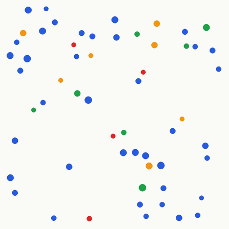
On this image Claude Haiku 5.5 answered 39 after listing the position of every dot. Qwen2-VL-2B said 40 and SmolVLM-256M said 14.
The models: SmolVLM-256M-Instruct (256M parameters, Apache-2.0) and Qwen2-VL-2B-Instruct (a 675M-parameter ViT plus a 1.5B language model, Apache-2.0), in bf16 with greedy decoding and at most 8 new tokens; Claude Haiku 5.5 (claude-haiku-5-5, thinking disabled, up to 400 output tokens, 2,000 for dense) through the Batch API; and Claude Sonnet 5.5 (claude-sonnet-5-5, thinking set to between_tools, since it rejects disabled) on the counting and reading tasks at 224 to 896 pixels. Each prompt was the question plus a sentence asking for the answer alone, and no reply hit its token limit. Rates carry 95% Wilson intervals, and differences on the same items use a paired bootstrap, as in Measuring LLMs Part 3.
Swipe to pan the diagram, or tap it to zoom.
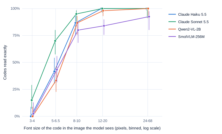
Reading needs pixels
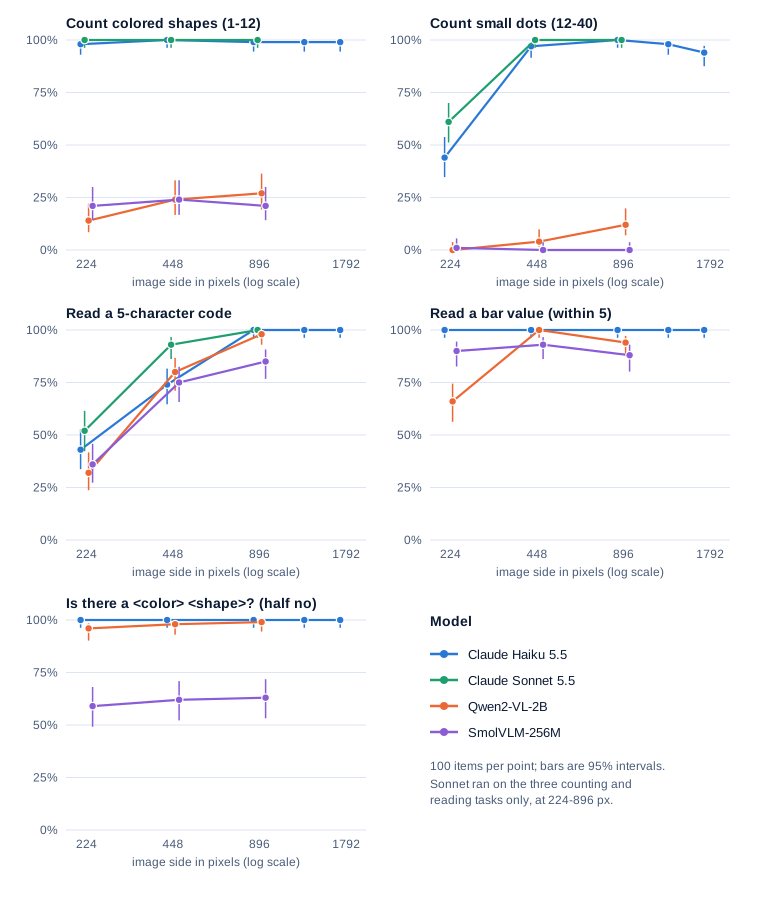
Haiku 5.5 read 43 codes of 100 at 224 pixels, 74 at 448 and every one from 896 up: +31 points from 224 to 448 (paired interval +22 to +40) and +26 from 448 to 896 (+18 to +34). The open models followed the same curve, Qwen2-VL-2B from 32 to 80 to 98 and SmolVLM-256M from 36 to 75 to 85.
Swipe to pan the diagram, or tap it to zoom.
What matters is the size of the letters in the image the model receives. At 3 to 4 pixels Haiku 5.5 and Qwen2-VL-2B read none of 40 codes. At 5 to 6.5 pixels Haiku read 42%, at 8 to 10 pixels 87%, and from 12 pixels up all of them; a Claude token covers 28 × 28 pixels, so at that size one token spans about three characters. On identical images Sonnet 5.5 read 52 codes at 224 pixels (9 more than Haiku, interval +1 to +17) and 93 at 448 (19 more, +12 to +27).
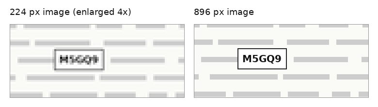
At 224 pixels, Haiku read this code as MSG09, Qwen2-VL-2B as M5009 and SmolVLM-256M as MSGB, confusing the shapes that blur together: 5 and S, Q and 0. Haiku declined 15 of the 100 codes at 224 pixels as too small to read.
Counting works because Haiku counts out loud
At 896 pixels Qwen2-VL-2B counted 1 to 12 shapes exactly 27 times in 100 and SmolVLM-256M 21, both tending to undercount. On 12 to 40 dots SmolVLM-256M got none right (median 11 too few), and Qwen2-VL-2B got 12 exact and 38 within 10%.
Haiku 5.5 got 99 of 100 shapes and 100 of 100 dots at 896 pixels. Its replies show how: with thinking disabled and an instruction to answer with a number only, it still wrote a coordinate for each object (“1. (170, 65) 2. (934, 122) …”) and then the total: a median of 67 output tokens for the shapes and 270 for the dots.
To test whether the list does the work, the 200 count and dense items went out again at 448 and 896 pixels with one added sentence: “Do not list, count aloud or explain: reply with the number immediately.” At 896 pixels, dense accuracy fell from 100% to 21%, a drop of 79 points (paired interval 71 to 87). Of the 94 replies that obeyed, answering in 10 tokens or fewer, 15 were right (16%, interval 10 to 25%); the 6 that listed anyway were all right. Shape counting at 896 pixels fell from 99% to 67%, and at 448 pixels dense counting fell from 97% to 40%.
The written list works like a chain of thought. Turning on Haiku’s own thinking (its default when the request leaves the setting out) added little on top of it: dense counts at 224 pixels went from 44% to 50% (+6, interval -2 to +14), and every task at 896 stayed at 99 to 100%. Sonnet 5.5 counted 61 dot images right at 224 pixels against Haiku’s 44 (+17, interval +7 to +27), and all 200 from 448 up.
Enlarged images add tokens and no accuracy
The 1,344 and 1,792-pixel images were enlarged 896-pixel ones, with two and four times the tokens. Haiku read every code at all three sizes, and on dense counts got 100, 98 and 94 right, so four times the tokens made it 6 points worse (interval 2 to 11). SmolVLM-256M’s default does this enlargement to every image, and its 224-pixel images, at 1,088 tokens, were read 36% of the time.
Tokens matter when they carry real pixels. The same 896-pixel images squeezed into one 512-pixel SmolVLM tile, 64 tokens, were read 33% of the time against 85% at 1,088 tokens (paired difference 52 points, interval 42 to 62). Counting, charts and the absent test didn’t change beyond noise.
Saying yes to things that aren’t there
Haiku 5.5 correctly said no to all 250 absent objects across five sizes, and Qwen2-VL-2B said yes to 1 of 50 at each size. SmolVLM-256M said yes to 23 of the 50 absent objects at 896 pixels (46%, interval 33 to 60%) while missing 14 of the 50 present ones: 63% accuracy, not far above a coin toss.
Reading charts
Haiku 5.5 read the exact value on all 500 chart items, with gridlines only every 20 units. Qwen2-VL-2B was within 5 on all 100 at 448 pixels but exact on 48; at 896 pixels all 6 of its misses were bars of height 5, read as 60 or 70. SmolVLM-256M stayed near 90% within 5.
How VLMs are evaluated
Public benchmarks test the same two things at scale, seeing and reasoning. The scores below are reported by the papers cited, not reproduced here.
POPE (Li et al., 2023), the Polling-based Object Probing Evaluation, measures object hallucination, a model describing objects that aren’t in the image. It asks Is there a/an <object> in the image? about 500 MSCOCO validation images, 6 questions each, half of them about absent objects. Those are drawn at random, from the dataset’s most common objects, or from objects that often appear alongside the real ones (adversarial). In the adversarial setting the original LLaVA scored 50.77% and answered yes 99.10% of the time; LLaVA-1.5-7B reports adversarial F1 (a balance of precision and recall) of 84.2. SmolVLM-256M’s 46% false-yes rate above is the same failure on synthetic shapes.
MMMU (Yue et al., 2023) tests reasoning: 11.5K college-level questions from exams, quizzes and textbooks across 30 subjects and 183 subfields, with charts, maps, music sheets and chemical structures. At release GPT-4V scored 56% and Gemini Ultra 59%, and extra pixels barely move it. In the Qwen2-VL paper’s ablation, Qwen2-VL-7B scored 53.33 on MMMU with 64 image tokens and 53.44 with 3,136, while InfoVQA, a test of reading infographics, rose from 28.85 to 77.27.
In the real world
- The SmolVLM paper reports 0.8 GB of GPU memory at batch size 1 for SmolVLM-256M and an MMMU score of 29.0%, against 42.0% for SmolVLM-2.2B; the Qwen2-VL paper gives Qwen2-VL-2B 41.1 on MMMU’s validation set.
- Claude caps image tokens at 4,784 on the high-resolution tier, so a 4K screenshot costs about what a 1,932-pixel square does. The docs suggest downsampling when the detail isn’t needed, since high resolution “can use up to roughly three times more visual tokens.”
- Open VLMs expose the knob: Qwen2-VL’s processor takes
min_pixelsandmax_pixels, SmolVLM’slongest_edge. On SmolVLM-256M, that one setting moved reading accuracy on the same images by 52 points. - Claude’s docs list counting (“especially with large numbers of small objects”) and images “under 200 pixels” among its limitations, which is where the experiment found the failures.
Common misconceptions
- “A bigger image always gives the model more to work with.” Only if the pixels are new. Enlarged copies cost four times the tokens and counted dots slightly worse.
- “Counting is a perception problem, so it either works or it doesn’t.” Haiku 5.5’s dense counts went from 100% to 21% when it was told not to list the dots.
- “Turning on thinking fixes what the model can’t see.” Reasoning can’t recover pixels that were never sent. With thinking on, Haiku read 44 codes at 224 pixels instead of 43.
- “A model that answers fluently has looked at the image.” SmolVLM-256M confirmed 46% of objects that weren’t there, in perfectly formed one-word answers.
- “Token count measures how much the model sees.” SmolVLM packs 1,024 patches into 64 tokens and BLIP-2 puts any image into 32. Detail depends on the pixels the encoder gets, not on the token count alone.
Key takeaways
- A VLM’s connector projects every patch into the language model’s input (LLaVA), summarizes the image into a fixed set of tokens (BLIP-2’s 32, Flamingo’s 64), or lets the language model cross-attend to it from inside.
- Large images get in by tiling, native resolution or pixel shuffle. Check your processor’s settings: SmolVLM’s default makes every image 1,088 tokens.
- On Claude an image costs its 28-pixel patch count plus 3 tokens, capped at 4,784, which is $0.0034 to $0.24 per 1,000 images on Haiku 5.5 in batch.
- Reading depends on letter size in the image the model gets: at 3 to 4 pixels the models read 0 to 15% of codes, and from 12 pixels up both Claude models read them all.
- Haiku 5.5 counts well because it lists every object; told to answer at once, it got 16% of dense counts right. A 256M-parameter model says yes to objects that aren’t there almost half the time.
What’s next
So far the series has been about understanding images. Part 5 starts generating them: the math of diffusion from scratch, how a model learns to undo noise one small step at a time, and a tiny diffusion model trained on this laptop’s GPU.
Further reading
- Visual Instruction Tuning (Liu et al., 2023): LLaVA, the linear projector and GPT-generated instruction data.
- Improved Baselines with Visual Instruction Tuning (Liu et al., 2023): LLaVA-1.5’s MLP connector, its 558K + 665K training data and POPE scores.
- BLIP-2: Bootstrapping Language-Image Pre-training with Frozen Image Encoders and Large Language Models (Li et al., 2023): the Q-Former and its 32 learned queries.
- Flamingo: a Visual Language Model for Few-Shot Learning (Alayrac et al., 2022): the Perceiver Resampler, gated cross-attention and per-image masking.
- Qwen2-VL: Enhancing Vision-Language Model’s Perception of the World at Any Resolution (Wang et al., 2024): native dynamic resolution, 2D RoPE in the ViT, three training stages and the image-token ablation.
- LLaVA-OneVision: Easy Visual Task Transfer (Li et al., 2024): AnyRes tiling and its token formula.
- SmolVLM: Redefining small and efficient multimodal models (Marafioti et al., 2025): pixel shuffle, image splitting and what small VLMs need.
- Evaluating Object Hallucination in Large Vision-Language Models (Li et al., 2023): POPE and its random, popular and adversarial settings.
- MMMU: A Massive Multi-discipline Multimodal Understanding and Reasoning Benchmark for Expert AGI (Yue et al., 2023): college-level multimodal questions across 30 subjects.
- Vision and Coordinates and bounding boxes (Claude API docs): the visual-token formula, resolution tiers, resize rule and limitations.
- SmolVLM-256M-Instruct and Qwen2-VL-2B-Instruct (Hugging Face model cards): the two local models used here, both Apache-2.0.