
Beyond Text: Images, Speech and Video · Part 2 of 13
Vision Transformers: Patches, Positions and Pixels, Measured
How a vision transformer turns images into tokens, what its position embeddings and attention learn, and what resolution and data cost, measured on a laptop.
On this page
TL;DR
A vision transformer (ViT) cuts an image into square patches, turns each patch into a vector with one strided convolution, adds a learned position vector to each, and runs the same Transformer blocks a language model uses. This part opens up Google’s ViT-B/16 on a laptop GPU. Its position vectors learned the image grid on their own and stretch to larger images far better than to smaller ones. Cost grows with the square of the image side, and attention’s share of it grows faster still. Attention starts local and widens with depth, and some tokens get repurposed as scratch space. Trained from scratch on a small dataset, a ViT loses badly to a convolutional network of the same size, which is why ViTs needed hundreds of millions of images, or heavy training tricks, to win.
Why it matters
Remove the position information from a pretrained ViT and its accuracy on 2,386 pet photos falls from 89.4% to 21.8%. Without the numbers that say where each of its 196 tiles came from, the model mostly can’t put the picture back together.
Resolution is the other pressure point. Feed the same model a 1024-pixel image instead of a 224-pixel one and it processes 4,097 tokens instead of 197, does 38 times the arithmetic, and runs 32 times slower on an RTX 4060 laptop GPU. A ResNet-50 convolutional network slows down only 19 times.
Both facts matter for the rest of this series, because the vision encoder in a vision-language model (Part 4) is usually a ViT, and its handling of position and resolution decides how many image tokens you pay for and what detail survives. Fundamentals Part 15 introduced patches and the original ViT result. This part measures what the pieces compute, what the trained model has learned, and what each choice costs.
The intuition
Picture a jigsaw puzzle with each piece’s grid coordinates written on the back. Spread the pieces anywhere and a helper who reads the coordinates can still reassemble the picture, comparing any piece with any other in a single glance, however far apart they started.
That is a ViT. The pieces are patches, the coordinates on the back are position embeddings, and the “compare any piece with any other” step is self-attention (Fundamentals Part 6).
A convolutional neural network (CNN) instead slides a small window across the image and builds a wider view by stacking many such windows, so locality is built into its wiring. A ViT has to learn from data that neighboring patches usually belong together.
The analogy breaks in two places. A puzzle helper reads the coordinates perfectly from the start, while a ViT begins with random position vectors and must learn what they mean. And the pieces aren’t fixed: at every layer each patch’s vector is rewritten using what it attended to, so by the last layer a “patch” carries information about the whole image.
Step 1: an image becomes 197 tokens
The patch embedding is a convolution
ViT-B/16, the “Base” model with 16-pixel patches, takes a 224 × 224 RGB image and cuts it into a 14 × 14 grid of patches. Each patch holds 16 × 16 × 3 = 768 numbers. A learned 768 × 768 matrix maps each flattened patch to a 768-number vector, the model’s width.
Fundamentals Part 15 wrote this as reshape-then-multiply. Real implementations write it as a convolution, a sliding filter, with a 16 × 16 kernel and a stride of 16, so the windows tile the image without overlapping. The two are the same computation, which this listing checks:
import torch

conv = torch.nn.Conv2d(3, 768, kernel_size=16, stride=16)   # ViT-B/16's patch embedding
x = torch.randn(1, 3, 224, 224)                              # one RGB image

a = conv(x).flatten(2).transpose(1, 2)                       # (1, 196, 768)

p = x.unfold(2, 16, 16).unfold(3, 16, 16)                    # (1, 3, 14, 14, 16, 16)
p = p.permute(0, 2, 3, 1, 4, 5).reshape(1, 196, 3 * 16 * 16) # 196 flattened patches
b = p @ conv.weight.reshape(768, -1).T + conv.bias           # one matrix multiply

print(a.shape, (a - b).abs().max().item())
It prints torch.Size([1, 196, 768]) and a largest difference of about 3e-06, which is floating-point rounding. The convolution is a fast way to run 196 copies of one matrix multiply, and it is the only layer that sees raw pixels.
The class token, or the mean
One more learned vector goes in front of the 196 patches: a class token, marked [CLS], borrowed from the text model BERT. It belongs to no patch, but attention lets it read every patch at every layer, so its final vector works as a summary of the image, and a linear layer on top gives scores for the 1,000 classes of ImageNet, the standard photo-classification benchmark. That makes 197 tokens.
The alternative is global average pooling: drop the class token and average the 196 output patch vectors, as CNNs such as ResNet do. The ViT paper’s first attempt at averaging “performed very poorly”, but the gap disappeared once the learning rate was tuned; the two “work similarly well, but require different learning-rates”. Vision-language models skip the summary and pass all the patch vectors on to the language model.

After the patch embedding, nothing in the model knows it is looking at an image.
Step 2: what position embeddings learn, and how they stretch
The model learns the grid by itself
Attention treats its input as a set: shuffle the 197 vectors and the outputs shuffle the same way. So ViT adds a learned vector to each of the 197 positions, numbered 0 to 196 in reading order like a sentence. Nothing in that numbering says that patch 15 sits directly below patch 1.
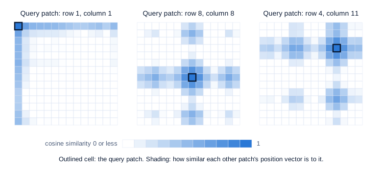
The ViT paper tried explicit 2D position embeddings and found no real gain. With ViT-B/16 and a linear classifier fit on five ImageNet examples per class, it scored 64.2% for plain 1D, 64.0% for 2D, against 61.4% with no positions at all. The reason shows up in the trained checkpoint. The chart takes three patches and shades every other patch by the cosine similarity (Fundamentals Part 4’s measure of how closely two vectors point the same way) between their position vectors.
Swipe to pan the diagram, or tap it to zoom.
The 1D numbering has become a 2D map. Averaged over all pairs, patches one step apart have position vectors with cosine similarity 0.68, two steps apart 0.34, and four steps apart about zero. Patches in the same row or column average 0.48; pairs that share neither average −0.06. Training on images taught the model rows and columns, which is why the hand-built 2D version added nothing.
To test how much the model relies on this, the experiment replaces all 196 patch position vectors with their average, so every patch gets the same one, and runs ViT-B/16 on the evaluation set used throughout this part: the 2,386 test images of the Oxford-IIIT Pet dataset (CC BY-SA 4.0) whose breed is also an ImageNet class, 24 breeds in all, scored with the model’s own 1,000-way ImageNet head. Accuracy fell from 89.4% (95% CI 88.1 to 90.6) to 21.8% (20.2 to 23.5).
Interpolating to a new resolution
A learned table has one problem: it has exactly 196 patch entries, for a 14 × 14 grid. Feed a 384 × 384 image and you get a 24 × 24 grid of 576 patches with no position vectors to match. The ViT paper’s fix is to treat the 196 vectors as a 14 × 14 image with 768 channels and resize it, with bicubic interpolation, to 24 × 24. The DeiT paper notes why bicubic rather than bilinear: bilinear blending shrinks the vectors’ length, and the pretrained network reacts badly to short vectors unless it is fine-tuned again.
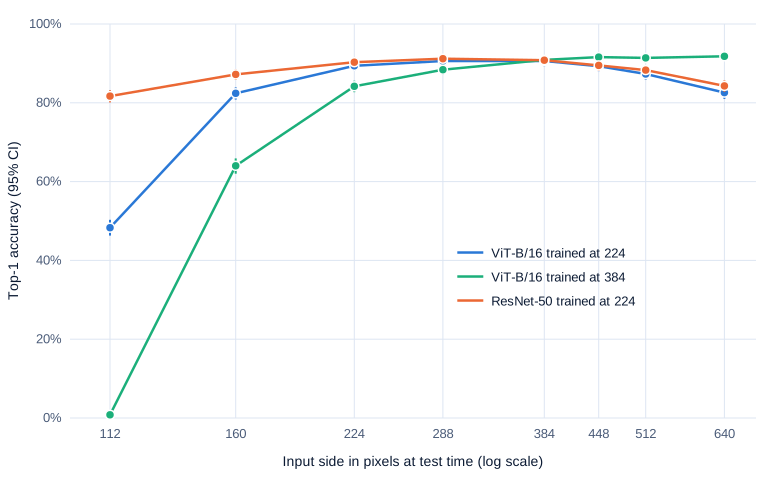
How well does that work with no fine-tuning? The next experiment runs three models at eight test resolutions on the same 2,386 images: ViT-B/16 trained at 224 pixels, the same architecture fine-tuned at 384 (google/vit-base-patch16-384), and a ResNet-50 CNN trained at 224 (microsoft/resnet-50), all Apache-2.0. Each image is resized on its shorter side and center-cropped to a square.
Swipe to pan the diagram, or tap it to zoom.
Stretching up works. The 224-trained ViT gains 1.2 points at 288 pixels (paired 95% CI +0.3 to +2.1), stays level at 384, and only drops off at 640, where the ResNet drops by a similar amount (−6.8 and −6.0 points from their 224 scores). The median image in this set is 500 × 375 pixels, so a 640-pixel crop is an upscale with blurry detail, and objects are bigger than anything the models trained on. Most of that loss comes from the images themselves, since the CNN has no position table and loses as much.
Shrinking fails. At 112 pixels the 224-trained ViT falls to 48.3%, while the ResNet keeps 81.7%. The 384-trained ViT, squeezed from a 24 × 24 table down to 7 × 7, scores 0.8%: 18 images right out of 2,386. Downsampling a smooth map of 576 learned vectors to 49 averages away the structure the model was trained to read, and the 384 model is the more fragile of the two at every size below its training resolution (−5.2 points at 224, CI −6.3 to −4.1).
Beyond a fixed table
Newer encoders avoid the fixed table. NaViT (Dehghani et al., 2023) learns separate row and column embeddings, trains on images at their native resolution and aspect ratio, and packs patches from several images into one sequence, masked so images can’t see each other. It matched the best fixed-resolution ViT with four times less compute.
Qwen2-VL’s 675M-parameter vision encoder (Wang et al., 2024) went further: it removed the absolute position embeddings and used 2D RoPE, rotary position embedding (Fundamentals Part 7) applied along two axes. Half of each attention head’s channels are rotated by an angle set by the patch’s row and the other half by its column, the “axial” scheme that Heo et al. (2024) compare against a learned-frequency variant. The rotation depends only on the row and column numbers, so any grid size works.
Step 3: what resolution costs
Tokens grow with the square of the side
Keep the 16-pixel patch and double the image side, and you get four times the patches. The token count is (side / 16)² + 1: 197 at 224 pixels, 785 at 448, 4,097 at 1024. Halving the patch size has the same effect.
Each Transformer block has two kinds of work. The linear layers (query, key and value projections, the output projection and the MLP) cost about 24 × N × D² floating-point operations (FLOPs) for N tokens of width D. GFLOPs below are billions of them. Attention’s two big matrix products, scores and weighted sum, cost 4 × N² × D. The first grows with N; the second with N². They are equal when N = 6D, which for ViT-B/16’s D = 768 is 4,608 tokens.
| Input side (pixels) | Tokens | Linear-layer GFLOPs per block | Attention GFLOPs per block | Attention share |
|---|---|---|---|---|
| 224 | 197 | 2.79 | 0.12 | 4% |
| 448 | 785 | 11.1 | 1.9 | 15% |
| 640 | 1,601 | 22.7 | 7.9 | 26% |
| 1024 | 4,097 | 58.0 | 51.6 | 47% |
At ImageNet sizes attention is a rounding error; at the resolutions vision-language models want for documents and screenshots, it is half the bill. PyTorch’s FLOP counter agrees: 35.1 GFLOPs for the whole model at 224 pixels, 1,320 at 1024.
Measured on a laptop GPU
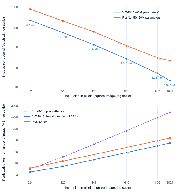
Both pretrained models were timed in half precision (fp16) on an NVIDIA GeForce RTX 4060 Laptop GPU (8 GB, PyTorch 2.11, CUDA 12.8) at six input sizes, with batch 16 for throughput and batch 1 for latency, reporting the median of 7 timed runs (15 for batch 1) after warm-up, with torch.cuda.synchronize() around each. During the ViT runs nvidia-smi read a median streaming-multiprocessor (SM) clock of 1,620 to 1,913 MHz and board power of 22 to 46 W, rising with input size (clocks and power limits left at defaults).
Swipe to pan the diagram, or tap it to zoom.
From 224 to 1024 pixels the image gains 20.9 times the pixels. ResNet-50’s throughput falls 19.4 times, nearly in proportion, because a CNN’s cost is linear in pixels. ViT-B/16’s falls 32 times, from 466 to 14.5 images per second (single-image latency 5.5 ms to 70 ms), and the extra is the N² attention term.
At small sizes the ViT holds up well. At 224 pixels it does 4.3 times the FLOPs of ResNet-50 (35.1 against 8.2 GFLOPs) yet is only 1.9 times slower, because its work is a few large matrix multiplies that keep the GPU’s tensor cores (its matrix-multiply units) busy: about 16 trillion FLOPs per second achieved, against 7 for the ResNet’s many small convolutions.
The memory chart shows attention’s cost most directly. Written plainly, attention stores a full N × N score table for each of the 12 heads, so one 1024-pixel image needs 1,574 MB of activations. PyTorch’s fused attention (scaled_dot_product_attention, a FlashAttention-style kernel) never stores that table and needs 73 MB, 21 times less, which is less than ResNet-50’s 120 MB. Fused attention is what makes high-resolution ViTs practical, though it removes only the memory, not the N² arithmetic.
Step 4: what the layers look at
Attention widens with depth
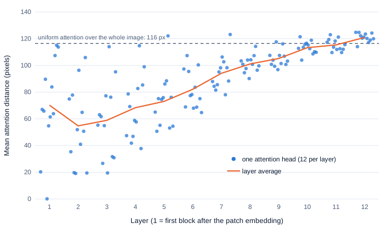
A CNN’s receptive field, the region of input one unit can see, grows layer by layer by construction. A ViT can attend across the whole image from layer 1; the question is whether it does. The ViT paper measured mean attention distance: for each query patch, the average pixel distance to the patches it attends to, weighted by the attention weights. Here it is measured on ViT-B/16 for 256 pet images at 224 pixels, for each of its 12 layers × 12 heads.
Swipe to pan the diagram, or tap it to zoom.
The early layers mix two kinds of heads. In layer 1, one head averages 0 pixels (each patch attends to itself), several sit at 20 to 65 pixels, and a few already spread over the whole image, above 110 pixels against 116 for uniform attention. With depth the local heads disappear: from layer 8 on, every head averages over 90 pixels, and in layer 12 all twelve sit between 114 and 125. The ViT paper found the same pattern in its larger models.
At 448 pixels, with interpolated positions, every distance roughly doubles (layer 12 average 241 pixels against 121): the heads cover the same share of the picture. The local early heads do the job of a CNN’s first layers, learned from data.
Tokens that become scratch space
Darcet et al. (2023) found something stranger in trained ViTs: a few patch tokens, usually in plain background, end up with vectors far longer than the rest. The model has repurposed them to “store, process and retrieve” global information, which leaves spikes in the attention maps. The fix is a few extra learned tokens, called registers, that belong to no patch and are discarded at the output, so the model has somewhere else to keep its notes.
The table counts these outliers in three checkpoints on 256 pet images, every 14th test image across all 37 breeds, flagging a patch token at the last layer whose vector length is more than 4 times the median.
| Model | Patch tokens over 4× median | Images with at least one | Largest/median at worst layer |
|---|---|---|---|
| ViT-B/16, supervised (ImageNet-21k, then ImageNet) | 5.4% | 256 of 256 | 42× (layer 7) |
| DINOv2 ViT-B/14 | 0.09% | 59 of 256 (95% CI 18% to 29%) | 60× (layer 9) |
| DINOv2 ViT-B/14 with 4 registers | 0% | 0 of 256 (CI 0% to 1.5%) | 3.3× (layer 1) |
The supervised ViT has them everywhere, about ten per image. DINOv2 without registers has rarer ones at the output but huge ones in the middle of the network, where its largest token is 60 times the median. The register version has none at any layer. The paper reports outliers for DINOv2 only at ViT-Large size and up; in this sample the Base model has them too, in fewer images.
Step 5: why ViTs needed so much data
Inductive bias versus data
An inductive bias is an assumption built into a model before it sees data. A CNN assumes that nearby pixels matter together and that a pattern means the same thing wherever it appears. Those assumptions usually hold for photos, so the network doesn’t have to learn them. The ViT paper puts it bluntly: in a ViT “only MLP layers are local”, and “all spatial relations between the patches have to be learned from scratch”.
Learning them takes data. The ViT paper’s ViT-B/32, slightly faster than ResNet-50, “performs much worse” when pretrained on a 9-million-image subset of Google’s private JFT-300M, and better from 90 million up. Only with 300 million images did ViT-H/14 beat the best CNNs, at 88.55% on ImageNet.
DeiT (Touvron et al., 2020) swapped data for training effort. On ImageNet’s 1.3 million images alone, with heavy augmentation (random image edits and blends such as RandAugment, Mixup and CutMix), stochastic depth (randomly skipping blocks during training) and 300 epochs, DeiT-B, the same 86M-parameter shape as ViT-B, reached 81.8% at 224 pixels after 53 hours on one 8-GPU machine, and 83.1% fine-tuned at 384.
A small run on the laptop
To see the data hunger directly, two models of the same size were trained from scratch on CIFAR-10, 60,000 labelled 32 × 32 photos in 10 classes (no license is stated on its home page; used only to train and measure, no images shown). The ViT has 3.2M parameters: 4 × 4-pixel patches (64 tokens plus a class token), width 256, 6 blocks, 4 heads. The CNN is a small ResNet-style network with 3.1M parameters. Both got the same recipe: the AdamW optimizer, 1,200 steps of batch 256 (about 6 epochs of the full set), cosine learning-rate decay, random crops and flips, bf16 (a 16-bit number format), on training subsets of 5,000, 15,000 and 50,000 images, with 2 seeds each, scored on the full 10,000-image test set.
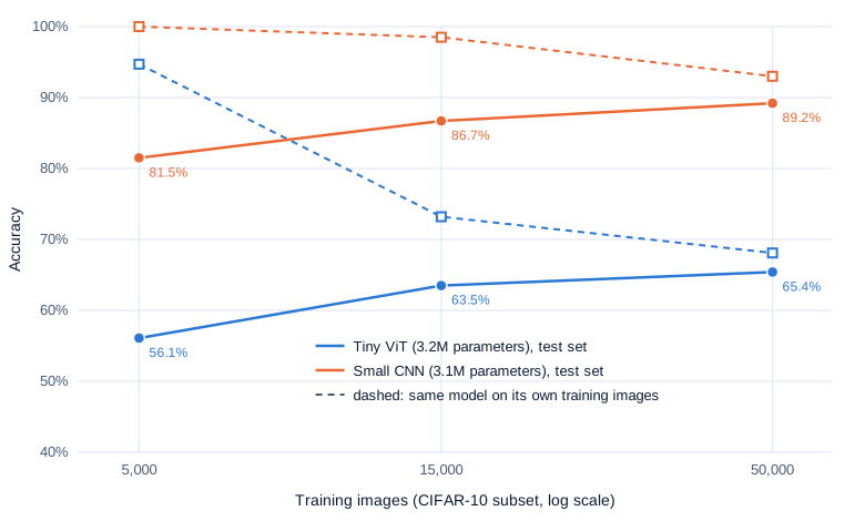
Swipe to pan the diagram, or tap it to zoom.
The CNN wins at every size, by 25.4 points on 5,000 images and 23.8 on the full 50,000. The two seeds never differ by more than 1.3 points and the test set adds about ±1 point of sampling error, so the gap is far outside the noise. The dashed lines show two different failures. On 5,000 images the ViT memorizes, scoring 94.7% on its own training images and 56.1% on new ones. On 50,000 it is still learning: 68.1% on its training images, barely above its test score, while the CNN already reaches 93.0%. With locality built in, the CNN gets more out of every image and every step.
A few laptop minutes can’t reach the crossover the ViT paper found, which took tens of millions of images. Going from 5,000 to 50,000 images raised the ViT by 9.3 points and the CNN by 7.7, a small hint of the same trend.
Learning without labels
The other route is to stop needing labels. Self-supervised learning trains on images alone, with a task the data sets for itself. DINOv2 (Oquab et al., 2023) trains a student ViT to match a teacher, a slowly updated average of the student itself, on different crops of the same image, and to predict the teacher’s features for patches it has had hidden. Its 1.1-billion-parameter ViT-g/14, trained on LVD-142M, a curated set of 142 million images, reaches 86.5% on ImageNet with a frozen network and only a linear layer trained on top.
In the real world
- The checkpoint measured here, google/vit-base-patch16-224 (86.6M parameters), was pretrained on ImageNet-21k (14 million images) and fine-tuned on ImageNet-1k, both at 224 pixels.
- DeiT’s Table 10 shows the same resolution trade at data center scale: one DeiT-B fine-tuned at 160, 224, 320 and 384 pixels scores 79.9%, 81.8%, 82.7% and 83.1% on ImageNet, while V100 throughput falls from 609 to 86 images per second (reported by Touvron et al., not reproduced here).
- Qwen2-VL uses one 675M-parameter ViT with 14-pixel patches and 2D RoPE for its 2B, 7B and 72B models, and merges each 2 × 2 group of output patches into one token, so a 224 × 224 image enters the language model as 66 tokens: 64 image tokens plus a start and an end marker (reported in the Qwen2-VL paper). Part 4 measures what such token counts cost.
- DINOv2’s register variants are published next to the originals, for example facebook/dinov2-with-registers-base (Apache-2.0, 4 registers).
Common misconceptions
- “A ViT has no convolutions.” Its first layer is one: a 16 × 16 filter with stride 16, the same computation as cutting patches and multiplying by a matrix. What it lacks is stacked small convolutions, and the built-in locality that comes with them.
- “Position embeddings tie a ViT to one resolution.” Interpolating the learned table worked with no fine-tuning: ViT-B/16 trained at 224 scored 90.6% at 288 and 384 pixels against 89.4% at 224. It fails in the other direction: shrinking a 384-trained table to a 7 × 7 grid dropped accuracy to 0.8%.
- “Attention is what makes ViTs expensive.” At 224 pixels attention is about 4% of ViT-B/16’s FLOPs. Its N² term reaches half the work only near 4,600 tokens, around 1,000-pixel images, though its memory explodes earlier unless a fused kernel is used.
- “ViTs are simply better than CNNs.” At equal size and small data a CNN wins clearly, as the CIFAR-10 run shows. ViTs win once data or training effort is large enough to learn what a CNN assumes.
- “Every token in a ViT describes its own patch.” Some background tokens get repurposed to hold global information, with vectors over 40 times the typical length, unless registers take that job.
Key takeaways
- A ViT is a Transformer encoder with one convolution in front: 16 × 16 patches become 196 vectors, plus a class token, plus a learned position vector for each.
- The 1D position vectors learn the 2D grid on their own, and the model leans on them heavily: removing them took accuracy from 89% to 22%. Interpolating them to a bigger grid works without retraining; shrinking them breaks the model.
- Tokens grow with the square of the image side and attention’s arithmetic with the square of the tokens, overtaking the linear layers near 4,600 tokens. Fused attention fixes the memory, not the compute.
- Attention is mixed local and global in early layers and global by the last ones, so the model learns some of a CNN’s locality from data.
- With little data a CNN beats a ViT of the same size, here by about 24 points on CIFAR-10 at every subset size; ViTs needed hundreds of millions of images, heavy augmentation, or self-supervised training like DINOv2 to pull ahead.
What’s next
A ViT trained on 1,000 ImageNet classes knows nothing about language. Part 3 trains a vision transformer and a text encoder together so a photo and its caption land on nearby vectors: CLIP’s contrastive loss, why it needs huge batches, and how it sorts images into categories it never trained on.
Further reading
- An Image is Worth 16x16 Words: Transformers for Image Recognition at Scale (Dosovitskiy et al., 2020): the ViT; patch embedding, position-embedding ablations and interpolation, data-scale experiments and mean attention distance.
- Training data-efficient image transformers and distillation through attention (Touvron et al., 2020): DeiT, a ViT trained on ImageNet alone; augmentation recipe, bicubic interpolation of positions and the resolution table.
- Vision Transformers Need Registers (Darcet et al., 2023): high-norm artifact tokens and the register fix.
- DINOv2: Learning Robust Visual Features without Supervision (Oquab et al., 2023): self-supervised ViTs trained on 142 million curated images.
- Patch n’ Pack: NaViT, a Vision Transformer for any Aspect Ratio and Resolution (Dehghani et al., 2023): native-resolution training with packed sequences and factorized position embeddings.
- Rotary Position Embedding for Vision Transformer (Heo et al., 2024): axial and learned-frequency 2D RoPE for ViTs.
- Qwen2-VL (Wang et al., 2024): a ViT encoder with 2D RoPE and dynamic resolution inside a vision-language model.
- Deep Residual Learning for Image Recognition (He et al., 2015): ResNet, the CNN used as the comparison here.
- The Oxford-IIIT Pet Dataset (Parkhi et al., 2012): the labelled photos used for the accuracy measurements (CC BY-SA 4.0).
- google/vit-base-patch16-224 model card: the checkpoint measured throughout this part.