
Beyond Text: Images, Speech and Video · Part 12 of 13
Video Generation: Spacetime Patches and Attention, Measured
How video models squeeze clips into spacetime patches, why attention cost explodes with clip length, and what temporal layers buy, measured on a laptop GPU.
On this page
TL;DR
Open video generators such as Wan, HunyuanVideo and CogVideoX squeeze a clip with a 3D autoencoder (4 times in time, 8 × 8 in space), cut it into spacetime patches, and run a diffusion transformer with flow matching over tens of thousands of tokens at once. This part counts those tokens, times full and factorized attention on a laptop GPU, trains four tiny video models that differ only in how frames talk to each other, and runs AnimateDiff, a motion module added to Stable Diffusion 1.5. Temporal attention keeps an object the same object from frame to frame, and letting every patch see every other patch costs the square of the clip’s length.
Why it matters
A five-second 720p clip from the open Wan 2.1 14B model takes 1,838 seconds on one H100-class GPU, per its model card. That is six minutes of a data-center GPU for every second of video, and the clip is 75,600 tokens long, 18 times what a 1024 × 1024 image costs Stable Diffusion 3.
By a rough count, about 70% of that arithmetic is attention, the step that lets each frame see the others. Trained here without attention across frames, a tiny video model made 1,500 clips and not one kept the same garment for 8 frames; its motion was as jerky as real frames shuffled at random. Switch off AnimateDiff’s motion modules and a fox walking through snow becomes 16 unrelated fox photos.
The intuition
Picture a flipbook drawn by a team. If each artist gets one page and never sees the others, every page is a good drawing, and flipping through gives a different cat on every page. That is an image model run frame by frame. If each artist can glance at the same spot on the other pages (factorized attention), the cat stays a cat and moves smoothly. If every artist can see every page at once (full spacetime attention), the whole book can be planned, but the meeting gets crowded fast: 80 artists make 6,400 pairs.
The analogy breaks in one place: a video model doesn’t draw page by page. Diffusion and flow models refine all the pages together, starting from noise, so the “talking” happens at every one of 25 to 50 refinement steps.
Step 1: a clip is a block of numbers that must shrink
Raw size
A video is a stack of frames, a 3D volume of pixels: time, height and width, each pixel with three color values. Five seconds at 16 frames per second and 1280 × 720 pixels, the default clip of the open Wan models (Wan team, 2025), is 81 frames, so
81 × 720 × 1280 × 3 = 223,948,800 numbersModels that only read video can sample a frame or two per second (Fundamentals Part 15); a generator has to produce every frame. Part 1 measured the image version: Stable Diffusion’s autoencoder squeezes a 512 × 512 picture 48 times, but run on every frame it took 2.1 seconds per second of video and ignored that neighboring frames are almost the same.
Causal 3D VAEs
So video models train their own variational autoencoder (VAE, a network that compresses an input into a small latent grid and decodes it back) that compresses time as well as space, with strikingly similar settings across labs:
| Model | Compression (time × height × width) | Latent channels | Source |
|---|---|---|---|
| CogVideoX | 4 × 8 × 8 | 16 | Yang et al., 2024, Table 1 |
| HunyuanVideo | 4 × 8 × 8 | 16 | Kong et al., 2024, Section 4.1 |
| Wan 2.1 | 4 × 8 × 8 | 16 | Wan team, 2025, Section 4.1 |
| Movie Gen | 8 × 8 × 8 | 16 | Movie Gen team, 2024, Section 3.1.1 |
The first three are causal: the encoder looks only at the current and earlier frames and keeps the first frame on its own, so 1 + T frames become 1 + T/4 latent frames (hence frame counts like 49, 81 and 129), and an image is just a one-frame video. CogVideoX’s authors found that at 16 × 16 × 8, “even if the channel dimensions are correspondingly increased, the convergence of the model also becomes extremely difficult.” For the Wan clip, 81 frames become 21 latent frames of 90 × 160 cells with 16 channels: 4,838,400 numbers, 46 times fewer than the pixels.
Spacetime patches
The transformer then cuts the latent into patches. OpenAI’s Sora report (Brooks et al., 2024) put the idea in one line: “we turn videos into patches by first compressing videos into a lower-dimensional latent space, and subsequently decomposing the representation into spacetime patches.” Those patches “act as transformer tokens”, and “this scheme works for images too since images are just videos with a single frame.” Wan and HunyuanVideo use 1 × 2 × 2 patches, so each token covers 4 frames and 16 × 16 pixels, the latent-space version of the tubelets Part 1 met in ViViT:
tokens = (1 + (frames − 1)/4) × (height/16) × (width/16)
Wan, 81 frames at 1280 × 720: 21 × 45 × 80 = 75,600 tokens| Clip | Model it matches | Tokens |
|---|---|---|
| 49 frames, 720 × 480 (6 s at 8 fps) | CogVideoX-5B | 17,550 |
| 81 frames, 832 × 480 (5 s at 16 fps) | Wan 2.1 1.3B | 32,760 |
| 81 frames, 1280 × 720 (5 s at 16 fps) | Wan 2.1 14B | 75,600 |
| 129 frames, 1280 × 720 | HunyuanVideo | 118,800 |
| 256 frames, 768 × 768, 8 × 8 × 8 then 1 × 2 × 2 | Movie Gen | 73,728 |
Only Movie Gen’s paper states its number (“∼73K”); the others are computed from each paper’s compression factors and each repository’s patch size. Stable Diffusion 3’s latent with 2 × 2 patches (Part 7) gives a 1024 × 1024 image 4,096 tokens; the 720p clip has 18 times as many, and 340 times as many pairs for attention to compare.

Step 2: who attends to whom
Full, factorized, and the arithmetic
Self-attention, where every token compares itself with others (Part 2 covers the image case), comes in two layouts for video. Full spacetime attention treats the clip as one sequence. With T latent frames of S patches each, there are (T × S)² pairs. Factorized attention, the older design, splits each layer in two: spatial attention within each frame (T sequences of S tokens), then temporal attention at each patch position across frames (S sequences of T tokens). For the Wan clip, T = 21 and S = 45 × 80 = 3,600:
full:        (21 × 3,600)²                 = 5.72 billion pairs
factorized:  21 × 3,600² + 3,600 × 21²     = 0.27 billion pairs
Factorized attention is 21 times cheaper, about a factor of T. The catch is reach: a patch reaches a different place in another frame only in two hops, along its frame, then along time. The whole difference is a reshape:
import torch
import torch.nn.functional as F

def attend(x, layout, heads=6):        # x: (batch, frames, patches, width) of query/key/value inputs
    B, T, S, D = x.shape
    if layout == "full":                # one sequence of T*S tokens
        seq = x.reshape(B, T * S, D)
    elif layout == "space":             # each frame alone: B*T sequences of S tokens
        seq = x.reshape(B * T, S, D)
    else:                               # "time": each patch position alone: B*S sequences of T tokens
        seq = x.transpose(1, 2).reshape(B * S, T, D)
    b, n, _ = seq.shape
    q = k = v = seq.reshape(b, n, heads, D // heads).transpose(1, 2)
    out = F.scaled_dot_product_attention(q, k, v).transpose(1, 2).reshape(b, n, D)
    return out.reshape(B, S, T, D).transpose(1, 2) if layout == "time" else out.reshape(B, T, S, D)

x = torch.randn(2, 8, 144, 192)         # 2 clips, 8 frames, 12 x 12 patches, width 192
for layout in ("full", "space", "time"):
    print(layout, tuple(attend(x, layout).shape))
Timed on a laptop
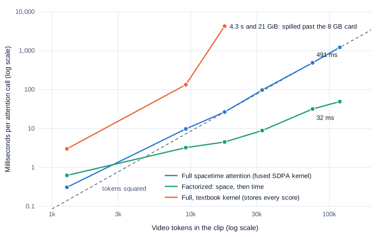
One attention call of 8 heads × 64 dimensions, in bf16 through PyTorch’s scaled_dot_product_attention (SDPA), was timed at the token counts of six clip sizes: the median of 7 timed calls after 3 warm-up, with torch.cuda.synchronize() around each, on an NVIDIA GeForce RTX 4060 Laptop GPU (8 GB, PyTorch 2.11, CUDA 12.8; median SM clock 2,175 MHz, clocks and power limits at their defaults).
Swipe to pan the diagram, or tap it to zoom.
| Clip (tokens) | Full attention | Factorized | Full ÷ factorized | Pair ratio |
|---|---|---|---|---|
| 1 s, 256 × 256 (1,280) | 0.31 ms | 0.63 ms | 0.5 | 4.9 |
| CogVideoX, 49 frames (17,550) | 26.7 ms | 4.5 ms | 5.9 | 12.9 |
| Wan 480p, 81 frames (32,760) | 98 ms | 8.9 ms | 11.0 | 20.7 |
| Wan 720p, 81 frames (75,600) | 491 ms | 32 ms | 15.4 | 20.9 |
| HunyuanVideo, 129 frames (118,800) | 1,224 ms | 49 ms | 24.8 | 32.7 |
From 17,550 tokens on, full attention follows the square law: 2.31 times the tokens (32,760 to 75,600) cost 5.0 times the time, against 5.3 predicted. It ran at 22 to 24 TFLOPS (trillion floating-point operations per second), close to the 25.3 that GPU Part 4 measured for this card’s 16-bit matrix multiplies, so the time is the arithmetic itself. Factorized attention falls short of its pair ratio because its many short temporal sequences keep the GPU less busy; for a 1-second clip it is slower than full attention.
PyTorch’s fused kernels, like FlashAttention (Inference Part 7), never store the score matrix, so the extra memory was just the output, 120 MiB at 118,800 tokens. The textbook kernel that keeps every score needed 5.8 GiB at 9,216 tokens and 21 GiB at 17,550, more than the 8 GB card holds; the WSL driver spilled it into system memory, and the call took 4.3 seconds, 160 times slower.
Scaled to Wan 14B’s real layer (40 heads of 128), one layer’s attention over 75,600 tokens is 4 × 75,600² × 5,120 ≈ 1.2 × 10^14 FLOPs, 4.9 seconds on this laptop. Over 40 layers that is 4.7 × 10^15 FLOPs per pass against about 2.1 × 10^15 for the weights (2 × 14 billion × 75,600), so attention is about 70% of the arithmetic. With 50 steps and two passes per step for guidance, the laptop would spend 5.4 hours on attention per clip, if the weights fit, which they don’t.
CogVideoX’s authors timed the same trade on an H800, 4.17 s per forward step at 768 × 1360 for 5 seconds with “2D+1D” attention against 9.60 s with 3D attention, and chose 3D anyway, because “this separated attention approach requires extensive implicit transmission of visual information, significantly increasing the learning complexity and making it challenging to maintain the consistency of large-movement objects.” In their ablation 2D + 1D attention was “unstable and prone to collapse.” Step 4 tests that claim at toy scale.
Step 3: video models grow out of image models
Reusing an image model
Captioned images are plentiful and captioned videos are not, so most of the field’s history is ways to reuse an image model.
- Video Diffusion Models (Ho et al., 2022) took an image U-Net and made it “factorized over space and time”: every 3 × 3 convolution became a 1 × 3 × 3 one that works within a frame, and “after each spatial attention block, we insert a temporal attention block that performs attention over the first axis and treats the spatial axes as batch axes.” Removing the temporal attention turns the model back into an image model, so it trained on images and videos together: adding 8 independent images per 16-frame clip cut FVD (a video quality score, Step 4) from 202 to 58 on 16 × 64 × 64 text-to-video samples.
- Make-A-Video (Singer et al., 2022) learned “what the world looks like and how it is described from paired text-image data, and … how the world moves from unsupervised video footage”, with no captioned video at all, adding temporal layers that start as the identity function.
- Video LDM (Blattmann et al., 2023) moved this into the latent space of Part 6’s Stable Diffusion: “the image backbone θ remains fixed and only the parameters ϕ of the temporal layers” are trained, about 650 million of them.
- AnimateDiff (Guo et al., 2023) inserts a motion module, a stack of temporal transformer layers, into a frozen Stable Diffusion 1.5, trained on WebVid-10M clips of 16 frames at 256 × 256 (per the paper’s first version) and “zero initialize[d]” so “the motion module is an identity mapping at the beginning of training.” Since the image weights never change, it animates any fine-tuned SD 1.5 checkpoint.
- Stable Video Diffusion (Blattmann et al., 2023) showed that data matters as much as layers: from 580 million clips (212 years of footage) it cut scenes at shot boundaries, dropped near-static clips by optical flow (the measured motion of pixels between frames), removed clips full of on-screen text and scored aesthetics with CLIP, keeping 152 million. A model trained on a curated quarter of a 10-million-clip sample beat one trained on the whole sample in human preference.
Then the backbone changed
Sora’s report described “a diffusion transformer” over spacetime patches whose sample quality “improves markedly as training compute increases.” The open models since then, Part 7’s DiT and flow matching scaled up, dropped factorization: CogVideoX uses “3D full attention”, HunyuanVideo “a unified Full Attention mechanism”, Movie Gen “full bi-directional attention”. Movie Gen, Wan and HunyuanVideo all train with flow matching; Wan defines its noisy input “as a linear interpolation between x0 and x1”, Part 7’s straight path.
AnimateDiff on a laptop
AnimateDiff’s motion module for SD 1.5, mm_sd_v15_v2.ckpt (1.82 GB), comes from guoyww/animatediff under Apache-2.0; the diffusers-format copy states no license on its card, so the original file is used. It adds 453.2 million parameters to Part 6’s Stable Diffusion 1.5 U-Net (CreativeML OpenRAIL-M), 1,312.7 million in all. This listing makes one 16-frame clip:
import torch
from diffusers import AnimateDiffPipeline, DDIMScheduler, MotionAdapter, UNet2DConditionModel, UNetMotionModel
from huggingface_hub import hf_hub_download

SD = "stable-diffusion-v1-5/stable-diffusion-v1-5"
ckpt = hf_hub_download("guoyww/animatediff", "mm_sd_v15_v2.ckpt")           # motion module, Apache-2.0
adapter = MotionAdapter.from_single_file(ckpt, torch_dtype=torch.float16).to("cuda")
unet2d = UNet2DConditionModel.from_pretrained(SD, subfolder="unet", variant="fp16",
                                              torch_dtype=torch.float16).to("cuda")
torch.set_default_dtype(torch.float16)
with torch.device("cuda"):                       # build the video U-Net on the GPU, in fp16, not in host RAM
    unet = UNetMotionModel.from_unet2d(unet2d, adapter)   # SD 1.5's layers plus the temporal motion modules
torch.set_default_dtype(torch.float32)
del unet2d
pipe = AnimateDiffPipeline.from_pretrained(SD, unet=unet, motion_adapter=adapter, variant="fp16",
                                           torch_dtype=torch.float16).to("cuda")
pipe.scheduler = DDIMScheduler.from_config(pipe.scheduler.config, clip_sample=False, timestep_spacing="linspace",
                                           beta_schedule="linear", steps_offset=1)
frames = pipe("a sailboat on a calm lake at sunset, gentle waves", negative_prompt="low quality, blurry",
              num_frames=16, height=512, width=512, num_inference_steps=25, guidance_scale=7.5,
              decode_chunk_size=4, generator=torch.Generator("cpu").manual_seed(42)).frames[0]  # 16 PIL images
print(len(frames), frames[0].size)
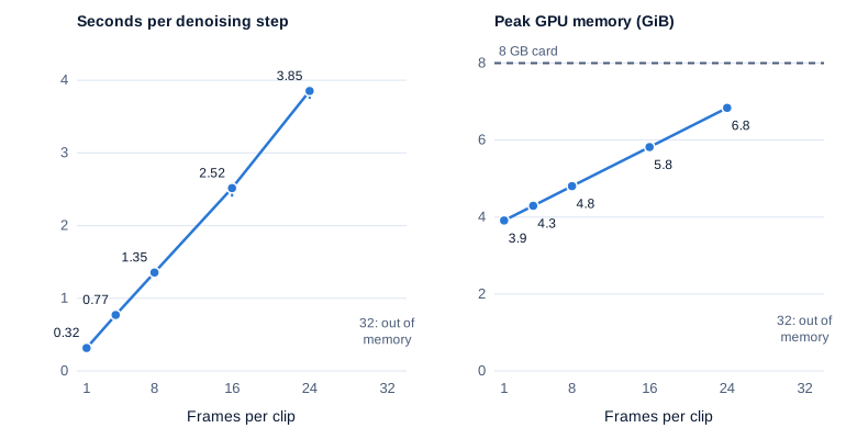
The torch.device("cuda") block matters on a small machine: merging the networks builds a fresh model, which on the CPU in fp32 is about 5 GB of host memory, and the first attempt here was killed by a 4 GB cap. Each step runs the U-Net on all frames at once, twice for guidance (median of 5 timed steps after 2 warm-up, SM clock 1,820 to 2,160 MHz, 41 to 48 W):
Swipe to pan the diagram, or tap it to zoom.
Each extra frame adds about 0.15 s per step and 0.13 GiB, so 32 frames ran out of memory. At 16 frames that’s 0.157 s per frame per step, 22% more than Part 6’s plain guided U-Net step (128.7 ms). A whole clip, 16 frames with 25 DDIM steps at guidance 7.5, took 67.5 to 70.4 seconds for each of four prompts (median 68.5 s, 6.4 GiB peak).
The motion modules are residual, output = input + temporal transformer(input), so returning the input switches them off and leaves plain Stable Diffusion denoising each frame from its own noise (47.0 seconds per clip).
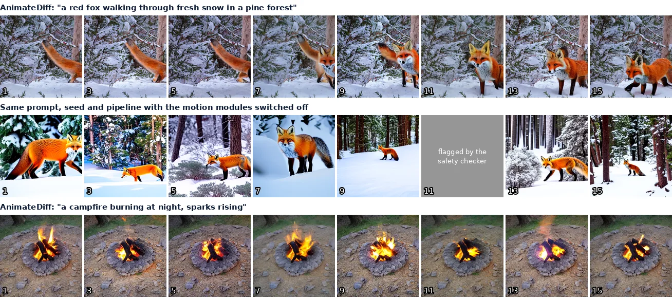
Between consecutive frames, CLIP image embeddings (openai/clip-vit-base-patch32, MIT) had a cosine similarity of 0.963 to 0.990 for the four AnimateDiff clips and 0.928 for both clips with the modules off, and the average pixel changed by 22 to 27 levels (out of 255) against 82 to 86.
The fox also shows a classic failure: it assembles itself as the clip runs, tail first and head later, the “spontaneous appearances of objects” that Sora’s report lists among its own failure modes. AnimateDiff’s pipeline has no safety filter, so SD 1.5’s checker ran on all 96 frames: it flagged none of the 64 AnimateDiff frames and 2 of the 32 motion-off frames, left out of the figure.
Step 4: what temporal attention buys, measured
The setup
Three small models were trained from scratch on synthetic clips: one Fashion-MNIST garment (Xiao et al., 2017, MIT license), 28 × 28 pixels, gliding across a dark 48 × 48 canvas for 8 frames at a random velocity of up to 3 pixels per frame on each axis, bouncing off the edges. Clips are generated on the GPU as training runs, so none repeats. All three are the same spacetime-patch transformer (4 × 4 patches, 144 per frame and 1,152 per clip, width 192, 6 adaLN-Zero blocks from Part 7, fixed sine-cosine positions in space and time) and differ only in attention:
| Model | Attention in each block | Parameters | Training time (4,000 steps) |
|---|---|---|---|
| Frame by frame | spatial only: every frame is generated on its own, like an image model | 4.17M | 366 s |
| Factorized | spatial, then temporal across the 8 frames at each patch position | 5.72M | 709 s |
| Full | one attention over all 1,152 tokens | 4.17M | 441 s |
Each trained with Part 7’s rectified flow loss for 4,000 steps of 32 clips (AdamW at 3e-4, bf16, torch.compile) and sampled with 32 Euler steps from an exponential moving average of its weights.
What to measure
Each frame’s garment is located (the bounding box of bright pixels), cropped to 28 × 28 and passed to the Fashion-MNIST classifier behind Part 5’s FD-FMNIST metric (91.1% test accuracy). That gives:
- Per-frame quality: FD-FMNIST, the Fréchet distance between classifier features of the crops and of the 10,000 test images (lower is better).
- Label consistency: does the classifier give all 8 frames the same class?
- Similarity: the cosine similarity of each frame’s classifier features to frame 1’s, the recipe of VBench’s subject consistency (below) with a tiny network.
- Motion: the garment’s speed in pixels per frame, and its jerkiness, the average change in velocity from frame to frame (0 for constant velocity, except at bounces).
Real test-set clips calibrate the scale, and so do “shuffled” clips whose 8 frames come from 8 different real clips.
Results
Each model generated 3 seeds of 500 clips. FD-FMNIST is the mean of the 3 seeds with their range; rates have 95% Wilson intervals over the 1,500 clips; the other columns are means whose 95% bootstrap intervals are within ±0.01 for similarity, ±0.06 for the motion of the trained temporal models, and ±0.25 for the two slideshows.
| Clips | FD-FMNIST per frame | Same class in all 8 frames | Similarity to frame 1 | Speed, px per frame | Jerkiness |
|---|---|---|---|---|---|
| Real test clips | 5.0 (4.6 to 5.4) | 98.8% (98.1 to 99.2) | 0.998 | 2.58 | 0.78 |
| Real frames, shuffled across clips | 5.0 (4.6 to 5.4) | 0.0% (0.0 to 0.3) | 0.500 | 10.9 | 18.9 |
| Frame by frame | 146 (144 to 148) | 0.0% (0.0 to 0.3) | 0.632 | 9.9 | 17.2 |
| Factorized | 195 (190 to 201) | 1.9% (1.3 to 2.7) | 0.811 | 2.30 | 1.57 |
| Full | 253 (248 to 260) | 13.9% (12.3 to 15.8) | 0.911 | 2.13 | 1.43 |
| Factorized, inflated from frame by frame (1,200 steps) | 159 (155 to 164) | 0.8% (0.5 to 1.4) | 0.773 | 2.62 | 2.75 |
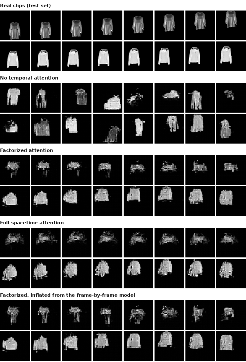
The frame-by-frame model makes the sharpest frames, and its clips are slideshows: no clip keeps one class, and its motion statistics match shuffled real frames.
Temporal attention fixes motion first. Both temporal models move their garment at close to the real speed (2.1 to 2.3 pixels per frame against 2.58), with jerkiness under 2 against 17 for the slideshow. Full attention beat factorized on every temporal measure and on training loss (0.090 against 0.103; frame by frame reached 0.117), CogVideoX’s argument at toy scale, and it trained faster, because at 1,152 tokens attention is cheap and the extra layers are not.
They paid in sharpness: capacity that the frame-by-frame model spent on single frames went into how frames relate, so their garments are blurrier (FD 195 and 253 against 146), which is also why the classifier’s label wavers on an obviously single blob. A fourth model was the factorized one inflated from the frame-by-frame model, with all its weights copied and the new temporal attention gated to zero, so at step 0 it was exactly the image model. After 1,200 steps (200 seconds) its frames were nearly as sharp (159), its garments moved at the right speed, and its loss, 0.100, was below what factorized reached from scratch in 4,000 steps; its motion was still jerkier. That is the bet behind Video LDM and AnimateDiff: keep what the image model knows and spend video training on time.
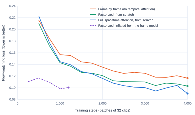
Swipe to pan the diagram, or tap it to zoom.
Scores for whole videos
FVD, the Fréchet Video Distance (Unterthiner et al., 2018), is the video version of Part 5’s Fréchet Inception distance, computed on features from I3D, a 3D convolutional network trained to recognize actions in Kinetics-400 YouTube clips. Because I3D sees whole clips, frames that are each fine but don’t fit together score badly. In the authors’ human study it agreed with raters 74.9% to 81.0% of the time where frame metrics couldn’t separate models, and “differences of 50 FVD or more typically seem to correspond to perceivable differences in the quality.”
VBench (Huang et al., 2023) splits quality into 16 dimensions with about 100 prompts each. Subject consistency is “the DINO feature similarity across frames”; background consistency uses CLIP; motion smoothness asks a frame-interpolation model to rebuild dropped frames; dynamic degree uses RAFT optical flow to check the video moves at all, since a still image repeated 16 times is perfectly consistent.
Physics
Physics is a separate problem. Sora’s report admitted it “does not accurately model the physics of many basic interactions, like glass shattering.” Physics-IQ (Motamed et al., 2025) filmed 396 real videos of 66 physical scenarios and asked models to continue them: the best scored 29.5 out of 100, and “visual realism is uncorrelated with physical understanding.” Kang et al. (2024) trained video diffusion models of 22M to 310M parameters on simulated moving balls: inside the training range the velocity error was 0.012 (0.010 on the real simulations), outside it 0.427, and the models generalized “case-based”, matching the nearest training example rather than learning the law.
In the real world
What one clip costs, from the models’ own papers, cards and READMEs (reported by their authors, not reproduced here):
| Model and license | Clip | GPU | Time per clip | Memory |
|---|---|---|---|---|
| CogVideoX-5B, CogVideoX License | 49 frames, 720 × 480, 50 steps | one H800 | 113 s | 26 GB |
| CogVideoX-5B | 5 s, 1360 × 768, 50 steps | one H800 | 500 s | 76 GB |
| Wan 2.1 T2V-1.3B, Apache-2.0 | 5 s, 832 × 480 | one RTX 4090, with offloading | about 4 minutes (261 s) | 8.19 GB |
| Wan 2.1 T2V-14B, Apache-2.0 | 5 s, 1280 × 720 | one H100 or H800 | 1,838 s | 69.1 GB |
| Wan 2.1 T2V-14B | 5 s, 1280 × 720 | eight H100 or H800 | 288 s | 29.9 GB per GPU |
| HunyuanVideo 13B, Tencent Hunyuan Community License | 129 frames, 1280 × 720, 50 steps | one GPU (type not stated) | 1,904 s | 60 GB peak |
- Text encoders are part of the bill: T5 v1.1 XXL for CogVideoX (per its repository config), umT5 with 5.3B parameters for Wan, a multimodal LLM for HunyuanVideo. They alone nearly fill or exceed this laptop’s 8 GB, which is why none of these models runs here.
- Movie Gen Video is a 30-billion-parameter transformer over “a maximum context length of 73K video tokens”, up to 16 seconds at 16 frames per second, trained on “up to 6,144 H100 GPUs”. Its paper gives no time per clip.
- Sora’s report gives no size or compute (“Model and implementation details are not included in this report”). Sora 2’s announcement claims it is “more physically accurate”, that a missed basketball shot now “will rebound off the backboard” instead of teleporting into the hoop, and that “the model is far from perfect and makes plenty of mistakes.”
Common misconceptions
- “A video model is an image model run on every frame.” Run frame by frame, the tiny model here made 1,500 clips and none kept one garment for 8 frames. Layers that work across time are what make a video model.
- “Factorized attention is always the cheap option.” It was 15 times faster than full attention at 75,600 tokens, but slower at 1,280, and the factorized tiny model trained 1.6 times slower than the full one, because short temporal sequences and extra layers keep the GPU less busy.
- “A consistent video is a good video.” A still image repeated 16 times is perfectly consistent, which is why VBench pairs consistency with a dynamic degree score. And consistency isn’t physics: the best model on Physics-IQ scored 29.5 out of 100.
- “Twice the length costs twice as much.” Full attention’s cost goes with the square: 2.3 times the tokens took 5.0 times as long.
Key takeaways
- Video models compress before they generate: a causal 3D VAE with 4 × 8 × 8 compression and 16 channels is the common choice, and 1 × 2 × 2 patches turn 5 seconds of 720p video into 75,600 tokens.
- Full spacetime attention costs the square of the token count. On a laptop GPU one attention call over 75,600 tokens took 491 ms against 32 ms factorized, and a 14B model does that 40 times per pass.
- The field moved from factorized space-time layers to full 3D attention once compute allowed. Even at toy scale, full attention learned consistent motion faster than factorized attention.
- Without temporal layers, frames don’t belong together. With them, motion and identity come first and sharpness lags, which is why video models start from image models: AnimateDiff adds 453 million temporal parameters to a frozen Stable Diffusion.
- Measure videos as videos: FVD on whole clips, VBench-style consistency together with how much the video moves, and physics separately.
What’s next
Images, sound and video all turn into tokens, and tokens cost money and time. Part 13, the finale, follows those costs into production: what image and audio tokens cost to serve, how caching encoder outputs saves work, and a look back at the whole series.
Further reading
- Video generation models as world simulators (Brooks et al., OpenAI, 2024): the Sora report; spacetime patches, the compression network and the limitations list.
- Video Diffusion Models (Ho et al., 2022): the factorized space-time U-Net and joint image-video training.
- Make-A-Video (Singer et al., 2022): text-to-video without captioned video, pseudo-3D layers initialized as the identity.
- Align your Latents (Blattmann et al., 2023): Video LDM, temporal layers trained on a frozen latent image model.
- AnimateDiff (Guo et al., 2023): the plug-in motion module run in Step 3; its first version gives the 16-frame, 256 × 256 training setup.
- Stable Video Diffusion (Blattmann et al., 2023): the data curation pipeline from 580 million clips to 152 million.
- CogVideoX (Yang et al., 2024): the 3D causal VAE, the expert transformer and the case against 2D + 1D attention, with timings.
- HunyuanVideo (Kong et al., 2024), Wan (Wan team, 2025) and Movie Gen (Meta Movie Gen team, 2024): three large open reports on full-attention flow-matching video transformers.
- Towards Accurate Generative Models of Video: A New Metric & Challenges (Unterthiner et al., 2018): FVD.
- VBench (Huang et al., 2023): 16 dimensions of video quality, including the consistency and motion measures used in Step 4.
- Do generative video models understand physical principles? (Motamed et al., 2025) and How Far is Video Generation from World Model: A Physical Law Perspective (Kang et al., 2024): physics tests for video generators.
- Model cards: Wan2.1-T2V-1.3B, CogVideoX-5b and the HunyuanVideo repository, for licenses, memory and time per clip.
- ViViT (Arnab et al., 2021): tubelet embedding and factorized attention for video understanding, the encoder-side ancestor of spacetime patches.
- Fashion-MNIST (Xiao et al., 2017): the garments in the synthetic clips (MIT license, Zalando Research).