
Beyond Text: Images, Speech and Video · Part 5 of 13
Diffusion From Scratch: Noise, Scores and a Laptop DDPM
The DDPM forward process, noise schedules, the noise-prediction loss and the score view, with a spiral and a Fashion-MNIST U-Net trained and measured.
On this page
TL;DR
A diffusion model learns one skill: look at a noisy picture and guess the noise in it. This article builds that from the ground up: the forward process and its one-jump formula, noise schedules and the signal-to-noise ratio, why a squared error on the noise is a reweighted likelihood bound, and the score view, in which denoising means walking uphill on the data’s log density. Then it trains a small network on a 2D spiral and a 1.6-million-parameter U-Net on Fashion-MNIST on a laptop GPU, and measures how sample quality depends on training, the noise schedule and the sampler: DDPM’s random steps or DDIM’s deterministic shortcut.
Why it matters
A network with 1.6 million parameters has only ever been asked one question: here is a piece of clothing with noise mixed in, what was the noise? After 13 minutes of that on a laptop GPU it draws sneakers, shirts and bags from pure static, at 183 images per second with 50 denoising steps, though it was never once asked to draw.
That trick, repeated, drives Stable Diffusion and the video generators of Part 12. Fundamentals Part 15 gave it a paragraph: start from noise, remove it step by step. This part opens the box: why a squared error on noise gives a model of the whole data distribution, and why the original method needed 1,000 steps when the same trained network can do with 20. On the laptop, the deterministic DDIM sampler with 20 steps scored 8.9 on our image-quality distance (lower is better), while DDPM’s random sampler still scored 10.4 with 50 steps and needed 100 to do better.
The intuition
Picture a drop of ink in a glass of water. Within minutes it spreads into a faint, even tint, and nothing about the tint tells you what shape the drop had. Physics never runs that film backwards. A diffusion model learns to: shown the tinted water at any moment, it learns which way each bit of ink most likely came from.
The forward direction needs no learning: add a little noise a thousand times until a picture is pure static. The backward direction is learned one small step at a time. The network is never asked to turn static into a sneaker in one go, only “which part of this is the noise?” Ask that a thousand times, starting from fresh static, and a picture appears that was never in the training set.
The analogy breaks in one place. Ink has a real past: there was one drop. Random static has no original to recover, so each backward step picks a plausible cleaner version, and the same static can end as a shirt or a bag depending on the sampler and the random draws along the way.
Step 1: burying data in noise, in one jump
The forward process is fixed; nothing in it is learned. Take a clean image with its pixels scaled to the range -1 to 1. At each of T = 1,000 steps, shrink the image slightly and add a little Gaussian noise, meaning random numbers drawn from the bell-shaped normal distribution with mean 0 and standard deviation 1, a fresh one for every pixel:
x_t = sqrt(1 - β_t) · x_(t-1) + sqrt(β_t) · ε ε ~ N(0, 1)β_t (beta) is the variance of the noise added at step t. Ho et al. raised it linearly from 0.0001 at step 1 to 0.02 at step 1,000, and that list of betas is the noise schedule. The shrink factor sqrt(1 - β_t) keeps the total variance near 1. Sohl-Dickstein et al. introduced the idea in 2015: “slowly destroy structure in a data distribution through an iterative forward diffusion process”, then “learn a reverse diffusion process that restores structure in data”.
Running 1,000 steps per training example isn’t needed: a sum of independent Gaussian kicks is itself Gaussian, so step t can be reached in one jump. Multiply the shrink factors together into , read “alpha bar t”. Then
In words: the clean image scaled by the square root of alpha bar, plus one draw of noise scaled by the square root of one minus alpha bar. The DDPM paper writes it as a distribution, . A check on one bright pixel, copied 100,000 times:
import numpy as np
T = 1000
betas = np.linspace(1e-4, 0.02, T)          # Ho et al.'s linear schedule
alpha_bar = np.cumprod(1 - betas)
rng = np.random.default_rng(0)
x0, t = 0.8, 300                             # one bright pixel, 300 noising steps
x = np.full(100_000, x0)                     # 100,000 copies of it
for b in betas[:t]:                          # the slow way: 300 small steps
    x = np.sqrt(1 - b) * x + np.sqrt(b) * rng.standard_normal(x.shape)
print(f"300 steps:   mean {x.mean():.4f}  std {x.std():.4f}")
ab = alpha_bar[t - 1]
print(f"closed form: mean {np.sqrt(ab) * x0:.4f}  std {np.sqrt(1 - ab):.4f}")
300 steps: mean 0.5064 std 0.7757
closed form: mean 0.5037 std 0.7769The two agree within sampling noise. After 300 steps a pixel that started at 0.8 is centered on 0.50 with a spread of 0.78, more noise than signal, and getting there cost one multiply and one add. That is what makes training cheap.
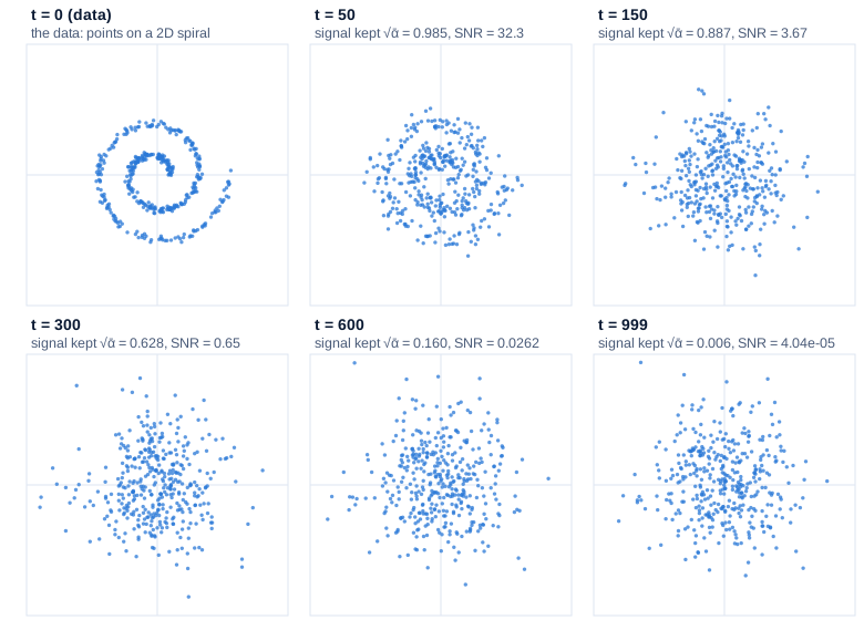
Swipe to pan the diagram, or tap it to zoom.
Signal-to-noise ratio and the schedule
How much of the data survives at step t comes down to one number, the signal-to-noise ratio (SNR): the variance of the signal part divided by the variance of the noise part, . At SNR 1 the image and the noise are equally strong; a schedule is a choice of how SNR falls from very high to nearly zero.
Nichol and Dhariwal noticed that the linear schedule “falls towards zero much faster, destroying information more quickly than necessary”, and that “the latents in the last quarter of the linear schedule are almost purely noise”. Their cosine noise schedule defines alpha bar directly as a squared cosine of t/T, with an offset s = 0.008 and each beta clipped at 0.999. Both, computed from the formulas:
| Step t of 1,000 | Linear: signal kept √ᾱ | Linear: SNR | Cosine: signal kept √ᾱ | Cosine: SNR |
|---|---|---|---|---|
| 1 | 1.000 | 10,000 | 1.000 | 24,200 |
| 100 | 0.947 | 8.7 | 0.986 | 34.8 |
| 250 | 0.724 | 1.1 | 0.920 | 5.5 |
| 500 | 0.280 | 0.085 | 0.703 | 0.98 |
| 750 | 0.058 | 0.0034 | 0.380 | 0.17 |
| 1,000 | 0.006 | 0.00004 | 0.000 | 0.000000002 |
| Share of steps with SNR below 0.01 | 32.6% | 6.4% |
A third of the linear schedule’s steps sit at an SNR below 0.01, where the image is less than a hundredth as strong as the noise. On one Fashion-MNIST boot:
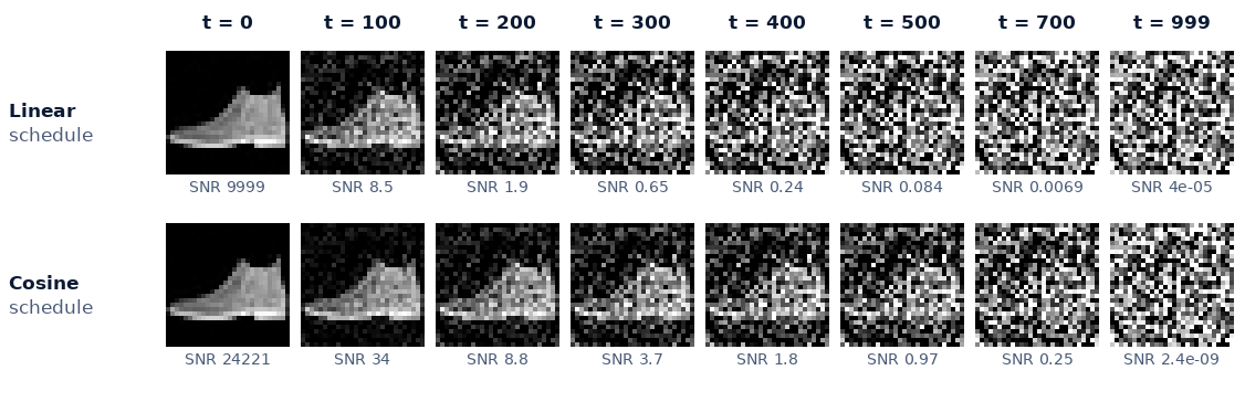
Nichol and Dhariwal found the linear schedule “sub-optimal for images of resolution 64 × 64 and 32 × 32”. Fashion-MNIST is 28 × 28; Step 4 tests both.
Step 2: what the network learns, and why it’s a squared error
The reverse process needs, at every step, a guess of what slightly cleaner image produced the current one. Ho et al. let a network predict the noise ε that was mixed in; θ (theta) stands for the network’s weights. Training is then four lines:
def loss_simple(model, x0, sched):
    t = torch.randint(0, sched.T, (x0.shape[0],), device=x0.device)   # a random noise level per image
    noise = torch.randn_like(x0)                                      # the answer key
    return F.mse_loss(model(sched.q_sample(x0, t, noise), t), noise)  # guess the noise, squared error
That is the paper’s “simplified” objective, equation 14:
In words: the squared distance between the true and predicted noise, averaged over steps, images and noise draws ( is the expected value from Math Part 4).
Where the squared error comes from
The principled way to train a probabilistic model is to maximize the probability it gives the training data, or a lower bound on it, the variational bound, when the exact probability is out of reach. For diffusion the bound splits into one term per step. Each term is a KL divergence (a measure of how different two distributions are) between the true one-step-back Gaussian, known exactly once x_0 is known, and the model’s guess. For two Gaussians with the same variance it reduces to a scaled squared difference of their means, which with the noise parameterization is proportional to ε minus ε_θ. Ho et al.’s equation 12:
weight(t) · || ε − ε_θ(x_t, t) ||² weight(t) = β_t² / (2 σ_t² α_t (1 − ᾱ_t))where α_t = 1 − β_t and σ_t² is the variance of the reverse step. So the bound is already a squared error on the noise, with a weight per step, and L_simple throws the weights away. With σ_t² = β_t and the linear schedule the weight is 0.50 at step 1, 0.074 at step 10 and 0.0055 at step 500: the bound puts 17% of its total weight on the first 10 of 1,000 steps, which only teach the removal of barely visible noise. Ho et al.: “our diffusion process setup in Section 4 causes the simplified objective to down-weight loss terms corresponding to small t”, “so that the network can focus on more difficult denoising tasks at larger t terms”. On CIFAR-10 (32 × 32 photos in 10 classes) the unweighted loss gave their best FID, 3.17, against 13.51 for the bound with fixed variances (Table 2; FID, the Fréchet Inception distance, is explained in Step 4). Reported, not reproduced here.
The score view: denoising is walking uphill
The score of a distribution is the gradient of its log density, : the direction in which the data becomes more likely fastest, the uphill direction from Math Part 7. For one noisy example it’s known exactly. x_t is the shrunken image plus noise of size sqrt(1 − ᾱ_t) · ε, so the direction back toward it is
score(x_t) = −ε / sqrt(1 − ᾱ_t)The predicted noise, flipped and rescaled, is an estimate of the score. In Song et al.’s words, “the DDPM training objective implicitly computes scores at each noise scale”. Sampling, read this way, starts in the blob and climbs the log density, a little less noisy at every step, until it reaches the data.
Song et al. (2020) let the number of steps go to infinity. The forward process becomes a stochastic differential equation (SDE), a rule for continuously adding noise, with an exact reverse-time SDE that “depends only on the time-dependent gradient field (a.k.a., score) of the perturbed data distribution”. The same paper derives a probability flow ordinary differential equation (ODE), with no randomness at all, a “deterministic process that samples from the same distribution as the SDE”. Every point of noise flows along a fixed curve to a point of data. DDIM is that picture in practice.
Step 3: sampling, the slow way and the shortcut
DDPM: ancestral sampling
DDPM’s sampler walks back one step at a time. It uses the predicted noise to estimate the clean image, , computes the mean of the true one-step-back distribution given that estimate, and adds a fresh draw of Gaussian noise with that distribution’s variance. This is ancestral sampling: each sample is drawn from its “parent” one step noisier. In the score picture it’s noisy hill-climbing, a step uphill plus a random kick, 1,000 times. The kicks let the chain correct its own earlier errors, and they make the endpoint a random function of the starting noise.
For fewer steps, take an evenly spaced subset of noise levels and treat each jump between neighbors as one step, with β = 1 − ᾱ_t / ᾱ_s for a jump from t down to s (Nichol and Dhariwal’s respacing).
DDIM: the deterministic shortcut
Song, Meng and Ermon’s DDIM (denoising diffusion implicit models) keeps the network and drops the kick. It estimates x̂_0 and ε̂, then rebuilds the image at the next noise level s with Step 1’s closed form, reusing the same noise:
x_s = sqrt(ᾱ_s) · x̂_0 + sqrt(1 − ᾱ_s) · ε̂It’s a valid sampler because the network was only ever trained on the one-jump distributions q(x_t | x_0), which DDIM leaves unchanged. The paper defines a family of samplers indexed by η (eta): η = 1 is DDPM’s ancestral sampler, η = 0 is DDIM. The update resembles “Euler integration for solving ordinary differential equations”, the simplest ODE solver, and a deterministic path can be followed with big steps; the paper reports samples “10× to 50× faster”.
What the paths look like
A 2D spiral makes both samplers visible. A multilayer perceptron (MLP: four fully connected layers of 256 units, 215,000 parameters, with a sine embedding of t) was trained on spiral points with the linear schedule, 20,000 steps of batch 1,024, on the CPU (about 4 minutes per seed).
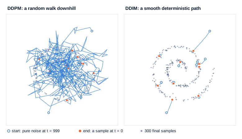
Swipe to pan the diagram, or tap it to zoom.
How many steps does the spiral need?
Three training seeds, two samplers, nine step counts, 5,000 samples each, two measures. The sliced Wasserstein distance projects both point clouds onto 500 random directions and averages how far apart the sorted projections are (0 means identical). The second is the share of samples within 0.1 of the noise-free spiral curve. Two independent sets of 5,000 real points score 0.017 (range 0.012 to 0.024 over 5 pairs) and 96.0%.
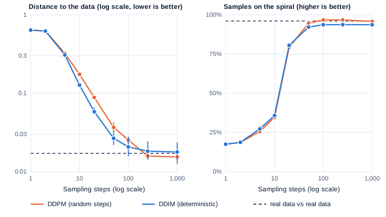
Swipe to pan the diagram, or tap it to zoom.
| Sampling steps | DDPM distance | DDIM distance | DDPM on spiral | DDIM on spiral |
|---|---|---|---|---|
| 1 | 0.64 | 0.64 | 17% | 17% |
| 10 | 0.174 | 0.127 | 35% | 36% |
| 20 | 0.088 | 0.058 | 79% | 81% |
| 50 | 0.037 | 0.027 | 95% | 92% |
| 250 | 0.016 | 0.018 | 97% | 94% |
| 1,000 | 0.015 | 0.018 | 96% | 94% |
| Real data (floor) | 0.017 | 0.017 | 96% | 96% |
One step gives a blob: the best single guess of x_0 from pure noise is near the average of the data, the spiral’s middle. At 10 and 20 steps DDIM is 27% and 34% closer to the data than DDPM, because its deterministic path tolerates big jumps. Past about 100 steps the order flips: DDPM reaches the floor with 97% of points on the curve, DDIM levels off at 94%. The random kicks that waste DDPM’s early steps also correct small errors that a deterministic path carries to the end. Nichol and Dhariwal saw the same on images: DDIM “produces better samples with fewer than 50 sampling steps, but worse samples when using 50 or more steps”. The seed spread is small next to these gaps: at 10 steps the DDPM seeds span 0.171 to 0.177, the DDIM seeds 0.121 to 0.136.
Step 4: a U-Net on Fashion-MNIST, trained on a laptop
Images need a network that sees shapes at several scales. DDPM uses a U-Net (Ronneberger et al., 2015): an encoder that shrinks the image to capture “context”, a decoder that grows it back for “precise localization”, and skip connections between levels of the same size. The output is one predicted noise value per pixel.

The time embedding lets one set of weights handle every noise level. The step number t becomes sines and cosines at 16 frequencies, the trick Transformers use for token positions, then a small MLP, and the result is added inside every residual block; Ho et al. “condition all layers on t” the same way.
| Setting | Value |
|---|---|
| Data | Fashion-MNIST training split, 60,000 grayscale 28 × 28 images in 10 classes (MIT license), scaled to -1 to 1 |
| Network | U-Net, 32/64/64 channels at 28/14/7 pixels, 2 residual blocks per level, attention at 7 × 7, dropout 0.1: 1.59M parameters, 0.55 GFLOP per image per call |
| Objective | L_simple (noise MSE), T = 1,000, linear or cosine noise schedule |
| Optimizer | AdamW, learning rate 5e-4 after 500 warm-up steps, batch 128, gradient clipping at 1.0 |
| Weights sampled | exponential moving average (EMA) of the weights, decay 0.9995 |
| Precision and speed | bf16 autocast, torch.compile; RTX 4060 Laptop GPU (8 GB), PyTorch 2.11 |
| Training | resumable chunks of at most 10.5 minutes; 11,500 steps per schedule (1.47 million examples, about 24 passes over the data) |
The exponential moving average is a slowly updated copy of the weights, moved 0.05% of the way toward the current weights each step, which smooths out training jitter.
Measuring sample quality: FD-FMNIST
Every sample set is scored with a Fréchet distance. A small classifier (a convolutional network trained on the Fashion-MNIST training split, 91.1% test accuracy) turns each image into 128 features. Fit a Gaussian, a mean vector and a covariance matrix, to the features of the generated set and another to the 10,000 test images, and measure the distance between the two Gaussians:
FD = |μ_gen − μ_test|² + trace(Σ_gen + Σ_test − 2 (Σ_gen Σ_test)^½)The first term compares the average image, the second the spread. It’s the recipe of Heusel et al.’s Fréchet Inception distance (FID), the standard image-generation metric, with our own classifier’s features instead of Inception-v3’s, so the numbers are not comparable with published FIDs. Call it FD-FMNIST; Part 7 and Part 8 use it too. Reference points: 2,000 real training images score 1.05 and 5,000 score 0.64 (the floor at each size, since a finite sample never matches perfectly); 5,000 images blurred with a 3 × 3 box filter score 73.8; uniform noise 718. Numbers below use 2,000 samples unless stated.
Training: the loss stalls, the samples don’t
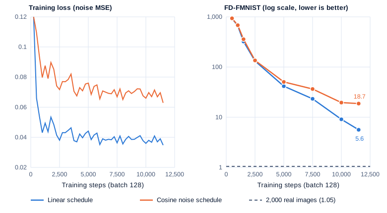
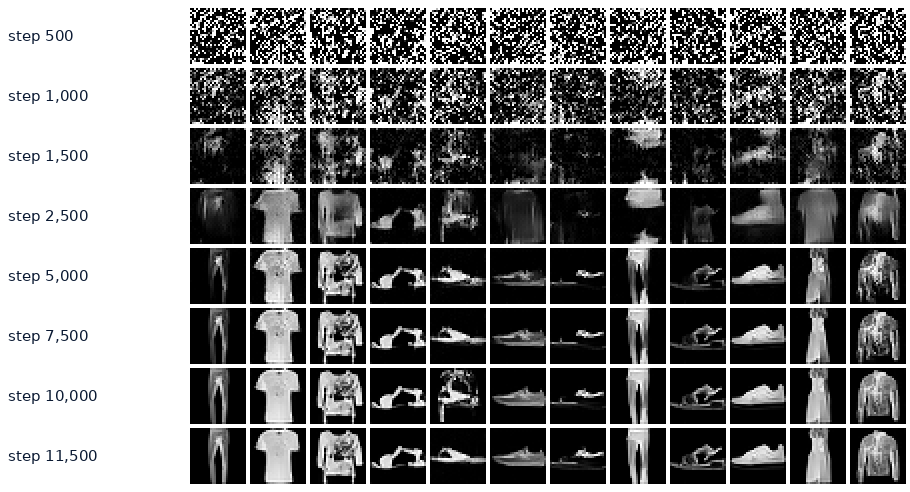
Both schedules trained for 11,500 steps with the same network, initialization and seed: 12.8 minutes of pure training for the linear run (two chunks, resumed once at step 6,750) and 9.3 for the cosine run, the gap being other jobs on the machine. Every 2,500 steps the script scored 2,000 EMA samples drawn with 50 DDIM steps.
Swipe to pan the diagram, or tap it to zoom.
Between steps 2,500 and 11,500 the linear model’s loss fell 8%, from 0.041 to 0.038, while FD-FMNIST fell 23 times, from 132 to 5.6. The loss averages over all 1,000 noise levels, and at high noise most of it is irreducible. Judged by the loss alone, training looked finished by step 3,000.
The cosine noise schedule lost here. It trailed from step 5,000 on, and at 11,500 steps scored 18.7 against 6.8 for the linear model with the same sampler and noise seed: the opposite of Nichol and Dhariwal’s ImageNet 64 × 64 result below. With one training seed per schedule, a small model and a short run, treat it as a result for this setup. Its higher loss, near 0.07, says nothing about quality: it spends more steps at low noise, where the exact noise in an almost clean image is hard to guess.
Sampling: steps, samplers and speed
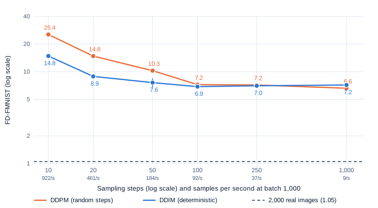
The final linear model sampled 2,000 images per setting, with the same starting noise for every setting:
Swipe to pan the diagram, or tap it to zoom.
| Sampling steps | DDPM FD-FMNIST | DDIM FD-FMNIST | Images per second at batch 1,000 | Time for one image alone |
|---|---|---|---|---|
| 10 | 25.4 | 15.0 (14.6 with a second noise seed) | 922 | 0.07 s |
| 20 | 14.8 | 8.9 | 461 | 0.13 s |
| 50 | 10.4 (10.1) | 6.8 (8.5) | 184 | 0.34 s |
| 100 | 7.2 | 6.9 | 92 | 0.67 s |
| 250 | 7.2 (7.2) | 7.0 | 37 | 1.7 s |
| 1,000 | 6.6 | 7.2 | 9 | 6.7 s |
Speeds are computed from the measured forward times below. The spiral’s pattern holds. At 10 steps DDIM’s distance is 41% lower than DDPM’s (15.0 against 25.4), and DDIM at 20 steps (8.9) beats DDPM at 50 (10.4). From about 100 steps both sit near 7 and the differences are within sampling noise: DDIM at 50 steps gave 6.8 and 8.5 with two noise seeds, and 5.6 with a third during training. DDPM with 1,000 steps was the best single number, 6.6, at 9 images per second. With 5,000 samples DDIM at 50 steps scored 5.66 against a floor of 0.64, so what’s left to improve is the model itself: more training or a bigger network.
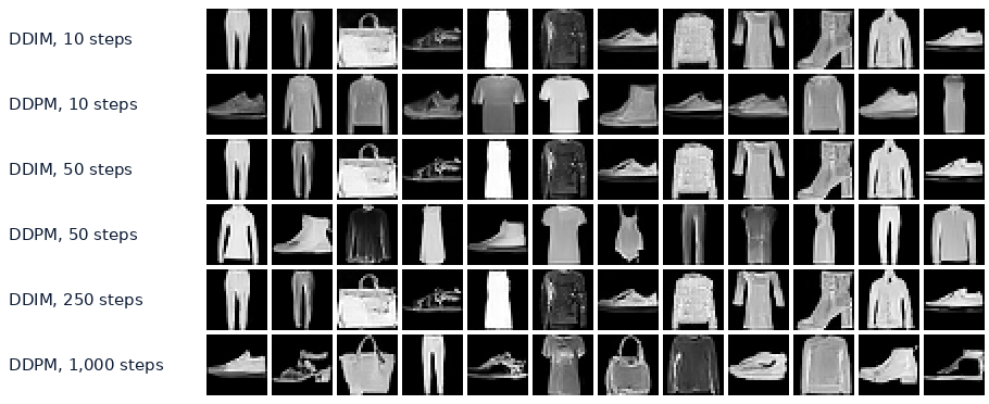
The DDIM paper calls this “consistency”. With the cosine noise schedule the sampler ranking flipped: DDPM led at 10 steps (28.4 against 38.6) and 50 (11.3 against 18.7). This run didn’t isolate why; one candidate is the last noise level’s SNR of 2 × 10⁻⁹, where turning predicted noise into an image estimate divides by a tiny number, an early error that DDPM’s fresh noise can wash out and DDIM carries to the end.
Timing (compiled bf16 model, CUDA synchronization, medians after warm-up): a forward pass takes 108.5 ms at batch 1,000 (7 runs of 20 calls), 11.0 ms at batch 100 and 6.7 ms for one image, and a 50-step DDIM batch of 1,000 takes 5.48 s (5 runs), the 183 images per second quoted above. The GPU ran at a median 1,710 MHz and 42.7 W. That is about 5 TFLOPS, a fifth of the 25.3 bf16 TFLOPS that GPU Part 4 measured on this card, because 32- to 64-channel convolutions underfeed the tensor cores; one image costs almost as much as a hundred because the GPU waits on kernel launches.
In the real world
- DDPM’s CIFAR-10 model: 35.7 million parameters, a U-Net with group normalization, self-attention at 16 × 16 and the sine time embedding “into each residual block”. It trained “at 21 steps per second at batch size 128 (10.6 hours to train to completion at 800k steps)” on a TPU v3-8, and “sampling a batch of 256 images takes 17 seconds”. FID 3.17. Reported by Ho et al., not reproduced here. The laptop model above is 22 times smaller and saw 70 times fewer training steps at the same batch size.
- DDIM on CIFAR-10 (Song, Meng and Ermon, Table 1): FID 13.36 with 10 steps against 41.07 for DDPM’s sampler (η = 1), 4.16 against 5.78 with 100 steps, and 4.04 against 4.73 with 1,000. DDPM with its larger variance reaches 3.17 at 1,000 steps but 367 at 10. The same crossover as on the spiral. Reported, not reproduced here.
- The cosine noise schedule: on ImageNet 64 × 64 with L_simple, 200,000 training iterations and T = 4,000, Nichol and Dhariwal report FID 27.0 with the cosine noise schedule against 31.3 with the linear one (Table 1). With learned variances, “100 sampling steps is sufficient to achieve near-optimal FIDs”. Reported, not reproduced here.
- Song et al.’s SDE models reached FID 2.20 on CIFAR-10 and generated 1024 × 1024 images. Karras et al. later pulled apart samplers, schedules and network preconditioning and reached FID 1.97 unconditional on CIFAR-10 “with much faster sampling (35 network evaluations per image)”. Reported, not reproduced here.
- Stable Diffusion keeps the noise prediction, the squared error and a time-conditioned U-Net, but runs them on an autoencoder’s 4 × 64 × 64 latent, which Part 1 measured at 48 times fewer numbers than its 512 × 512 picture.
Common misconceptions
- “The network removes all the noise in one pass.” Its one-shot guess from pure noise is near the average of the data. On the spiral, one sampling step put 17% of points on the curve against 96% for real data (distance 0.64 against 0.015 with 1,000 DDPM steps).
- “A lower training loss means better samples.” Between steps 2,500 and 11,500 the loss fell 8% while FD-FMNIST fell 23 times. The cosine run’s higher loss reflects which noise levels it spends time on and says nothing about its samples.
- “DDIM is a different model that needs its own training.” It’s a different sampler for the same weights. Every DDIM number here used the network trained with the DDPM loss.
- “More sampling steps always help.” DDIM was flat from 50 to 1,000 steps (6.8 to 7.2, within sampling noise) while the cost grew 20 times; DDPM crept to 6.6. The trained network set the floor.
- “The cosine noise schedule is always better.” Nichol and Dhariwal found it better on 64 × 64 ImageNet. On 28 × 28 Fashion-MNIST with this small U-Net, one run each, it was worse at every checkpoint from step 5,000 on. Schedules interact with resolution, model and training length; measure them.
Key takeaways
- The forward process has a closed form, so any noise level costs one multiply and one add. That is what makes training cheap.
- Predicting the noise with a squared error is the variational bound with its per-step weights removed, which shifts effort away from barely noisy images and gave Ho et al. better samples.
- The predicted noise is a scaled score, the uphill direction of the log density. DDPM climbs with random kicks; DDIM follows the deterministic probability flow ODE with the same network.
- On the laptop, DDIM with 20 steps (FD 8.9) beat DDPM with 50 (10.4), and at 10 steps it was 41% better. Past 100 steps both samplers stalled near FD 7 against a real-data floor of about 1, a limit set by the network.
- Score the samples themselves: the loss moved 8% while sample quality improved 23 times.
What’s next
Everything here ran on 28 × 28 pixels, and even that costs about 0.55 billion floating-point operations per network call per image. A 512 × 512 photo has 334 times as many pixels. Part 6 moves the same process into the compressed latent space of an autoencoder, adds a text prompt through cross-attention and classifier-free guidance, and times Stable Diffusion 1.5 on the same laptop GPU.
Further reading
- Denoising Diffusion Probabilistic Models (Ho, Jain and Abbeel, 2020): the forward closed form, the noise parameterization and L_simple, with the CIFAR-10 U-Net.
- Deep Unsupervised Learning using Nonequilibrium Thermodynamics (Sohl-Dickstein et al., 2015): the original diffusion model, forward diffusion and a learned reverse.
- Improved Denoising Diffusion Probabilistic Models (Nichol and Dhariwal, 2021): the cosine noise schedule, learned variances and respaced sampling.
- Denoising Diffusion Implicit Models (Song, Meng and Ermon, 2020): the deterministic sampler, the η family, and FID against steps.
- Score-Based Generative Modeling through Stochastic Differential Equations (Song et al., 2020): the score view, the reverse-time SDE and the probability flow ODE.
- Elucidating the Design Space of Diffusion-Based Generative Models (Karras et al., 2022): samplers, schedules and preconditioning pulled apart and tuned.
- U-Net: Convolutional Networks for Biomedical Image Segmentation (Ronneberger, Fischer and Brox, 2015): the contracting and expanding paths with skip connections.
- GANs Trained by a Two Time-Scale Update Rule (Heusel et al., 2017): where the Fréchet Inception distance comes from.
- Fashion-MNIST (Xiao, Rasul and Vollgraf, 2017): the dataset, MIT license, from Zalando Research.
- What are Diffusion Models? (Lilian Weng, 2021): the derivations in one place, with consistent notation.
- Generative Modeling by Estimating Gradients of the Data Distribution (Yang Song, 2021): the score view explained by its author.