
Measuring LLMs: Evals and Benchmarks · Part 3 of 11
The Statistics of Evals: Error Bars, Paired Tests and Power
A benchmark score is an estimate. 1,140 MMLU questions asked of Claude five times: error bars, clustered errors, paired tests, power and many comparisons.
On this page
TL;DR
A benchmark score is an estimate: the share of one sample of questions a model got right, standing in for how it would do on questions like them. This article measures how far to trust it, with 1,140 MMLU questions asked five times each of Claude Haiku 5.5. Asking again moved the score by at most 1.0 point, while the choice of questions sets an error bar of ±2.3 points, or ±4.2 once you allow for questions coming in subject groups. Comparing two systems on the same questions shrank the error bar on their difference by 20% to 36%, so a 3-point gap needs about 1,165 questions instead of 1,804 per system. On a simulated leaderboard of 20 identical copies of one model, 82% of leaderboards showed at least one “significant” gap when nothing corrected for the 190 comparisons.
Why it matters
Ask Claude Haiku 5.5 the same 1,140 exam questions five times and its score barely moves: 79.7%, 80.0%, 80.0%, 80.7%, 80.2%. Yet the questions were one draw from a much larger pool, and on a different draw of 1,140 the score could plausibly land anywhere from 75.5% to 84.0%.
Most reported scores come without any of this. Haiku 5.5’s own system card gives 87.8% on a multilingual MMLU from a single trial; a leaderboard might put two models half a point apart. Each is one number from a finite sample, with an uncertainty nobody wrote down.
The statistics for writing it down are old. Evan Miller’s Adding Error Bars to Evals (2024) collected them for language models, and Agentic AI Part 11 used them on 64 agent tasks. This part applies them to a knowledge benchmark, checks each formula by resampling real answers, and adds the leaderboard’s problem of many comparisons at once.
The intuition
Think of an opinion poll. A pollster calls 1,000 voters, reports 52% support and adds “a margin of error of 3 points”. The margin comes from which 1,000 voters happened to be called: call another 1,000 and the number moves.
A benchmark is a poll of questions. The score on 1,140 questions estimates the score on all questions like them, and its margin of error comes mostly from which questions were picked. Asking the same question twice is calling the same voter twice, which shows how firm that one voter is. Polling whole households widens the margin, because people in one house tend to agree, and questions from one subject behave the same way. To compare two candidates, you ask the same voters about both.
The analogy breaks in one place. A poll samples real voters, while a benchmark’s “all questions like these” is imaginary: MMLU’s questions were collected, never drawn at random from anything. An error bar says how much the score would move if the questions had come differently from the same kind of source. Whether that source measures what you care about is a separate question, the subject of Part 1.
Step 1: a score is an estimate
The setup
Every measurement here uses one fixed sample of MMLU, the Massive Multitask Language Understanding benchmark (Hendrycks et al., 2020, MIT license): 20 questions from each of its 57 subjects, 1,140 of the 14,042 in the Hugging Face copy of its test split (the paper counts 14,079), drawn once with seed 0 and shared with Part 4. Each question has four options and one right answer. One, from the “miscellaneous” subject:
Including the bottom how many sides are on a square-based pyramid?
A. three   B. four   C. five   D. six
The right answer is C. Haiku answered D four times out of five.
A system prompt asked for a single letter. The main configuration is claude-haiku-5-5 with thinking off (thinking: {"type": "disabled"}), max_tokens 16, no effort setting (the API default, medium) and no temperature setting, so answers are sampled the usual way. Each question was asked K = 5 times: 5,700 requests through the Message Batches API, for $0.067.
A reply counts as an answer if it starts with a letter. On 73 questions, mostly calculations, Haiku sometimes began working the problem out and hit the 16-token limit first. Those 333 replies (5.8%) score as wrong, as a strict harness would score them. Part 1 asked such replies again with room to finish and got 85.3% on these same questions; Part 4 is about choices like this one.
The standard error
The first run got 909 of 1,140 right: 79.7%. Score each question 1 (right) or 0 (wrong) and the score is the mean of those 1,140 numbers, an estimate of an expected value in the sense of Math Part 4. The Central Limit Theorem (CLT), the rule that an average of many independent random numbers is close to normally distributed, says how far that mean typically lands from the truth. That typical distance is the standard error (SE):
SE = sqrt( p (1 - p) / n ) = sqrt( 0.797 × 0.203 / 1,140 ) = 0.0119Here p is the score and n the number of questions. A 95% confidence interval, a range built so that 95 times in 100 it contains the true value, reaches about 1.96 standard errors either side: 79.7% ± 2.3 points, or 77.4% to 82.1%. Resampling the 1,140 questions 10,000 times with replacement, the bootstrap, gives 77.4% to 82.0%, so at this size the textbook formula holds.
How the error bar shrinks
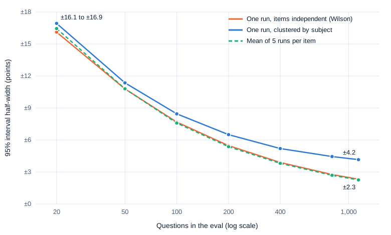
Because of the square root, four times the questions only halves the interval. The chart measures it on 300 random subsets of each size, drawn from the 1,140.
Swipe to pan the diagram, or tap it to zoom.
At 20 questions the error bar is ±16 points, at 100 it is ±7.7 and at 400 it is ±3.9; a 50-question eval can’t tell a 75% model from an 85% one. Step 2 explains why five answers per question barely beat one, and why the clustered line flattens: a growing subset keeps adding questions to the same 57 subjects.
Small evals need a better interval
The “±1.96 standard errors” interval, the Wald interval, assumes a roughly normal score, which fails with few questions or a score near 0% or 100%. Bowyer et al. (2025), a position paper titled “Don’t Use the CLT in LLM Evals With Fewer Than a Few Hundred Datapoints”, found that CLT-based methods then “perform very poorly, usually dramatically underestimating uncertainty”, and recommend a Wilson score interval or a Bayesian one instead.
Real answers can test that. Treat all 5,700 of Haiku’s answers as the population, whose true score is 80.1%. Draw a small eval at random, one answer per question, build each interval and count how often it contains 80.1%; a 95% interval should do so 95% of the time:
| Questions | Wald (±1.96 SE) | Wilson | Bootstrap |
|---|---|---|---|
| 10 | 88.7% | 96.8% | 86.1% |
| 20 | 92.1% | 95.5% | 89.9% |
| 30 | 93.6% | 96.0% | 91.8% |
| 50 | 93.7% | 95.4% | 93.4% |
| 100 | 93.4% | 94.1% | 94.0% |
| 200 | 94.3% | 94.6% | 93.7% |
Each cell is the share of 4,000 simulated evals whose interval contained the truth, accurate to about ±0.7 points. Below about 50 questions the Wald and bootstrap intervals are too narrow and the Wilson interval keeps its promise; from 100 up they agree.
Step 2: questions, not runs, are the unit
Splitting the variance
Five answers per question let the variance be split in two. Part of the spread in a graded answer comes from the question, since some are easy for this model and some hard. The rest comes from sampling: the same question, asked again, can get a different answer. Miller writes the variance of the benchmark mean as (Var(x) + E[σ²] / K) / n, where Var(x) is the spread of the questions’ true success rates, E[σ²] the average sampling variance of one answer to one question, and K the answers per question.
| Quantity | Haiku 5.5, thinking off |
|---|---|
Between questions, Var(x) | 0.149 |
Within a question, E[σ²] | 0.010 |
| Sampling’s share of the total | 6.4% |
| SE, one answer per question | 1.18 points |
| SE, five answers per question | 1.15 points |
Haiku is consistent: 889 questions right all five times, 203 wrong all five times, and 48 that changed. The five runs scored between 79.7% and 80.7%, and an exact McNemar test (Step 3) found no difference between any two of them; the smallest of the 10 p-values was 0.052. Miller’s worked example has resampling cut variance by up to two-thirds when answers vary a lot within each question, as long generations do. On multiple choice without thinking, nearly all the variance is in the questions.
Rerunning the same questions shows how consistent the model is, and nothing about the questions you didn’t ask, where nearly all the uncertainty lives. Agent tasks vary more between runs, so repeats paid off more in Agentic AI Part 11.
Clustered standard errors
The CLT formula assumes the 1,140 questions are independent. They come in 57 subjects of 20, though, and a model weak at a subject is weak at most of its questions. Haiku’s subject scores ran from 31% on abstract algebra to 100% on four subjects, including high school government and politics, and 17% of the variance in per-question success rates lay between subjects.
A clustered standard error lets questions in the same group be correlated. Miller’s equation 4 adds, for every pair of questions in the same subject, the product of their deviations from the mean:
import numpy as np

def clustered_se(s, groups):
    """Standard error of mean(s) when items in the same group may be correlated."""
    s, groups = np.asarray(s, float), np.asarray(groups)
    n, r = len(s), s - s.mean()
    cross = sum(r[groups == g].sum() ** 2 - (r[groups == g] ** 2).sum() for g in np.unique(groups))
    return np.sqrt(s.var(ddof=1) / n + cross / n**2)
On Haiku’s first run it returns 2.15 points against the naive 1.19, so the 95% interval widens from ±2.3 to ±4.2 points: 75.5% to 84.0%. The ratio of the two variances, 3.3, is called the design effect: 1,140 correlated questions carry about as much information as 350 independent ones. Resampling whole subjects instead of questions agrees, at 75.4% to 83.7%. Miller reports clustered standard errors “over 3X larger than naive standard errors” on DROP, a reading benchmark where many questions share one passage.
When to cluster
Which interval to report depends on the claim. “Haiku scores 79.7% on these 57 MMLU subjects” treats the subjects as fixed and fits the naive interval. “Haiku gets about 80% of academic exam questions right” treats them as a sample of possible subjects and needs the clustered one. Anthropic’s summary of Miller’s paper recommends “clustering standard errors on the unit of randomization”, whatever was drawn at random.
The cost of getting it wrong can be measured. Draw a few whole subjects at random, 20 questions each, and count how often each interval contains the 80.1% truth:
| Subjects drawn | Questions | Naive Wilson interval | Clustered interval |
|---|---|---|---|
| 5 | 100 | 70.4% | 79.7% |
| 10 | 200 | 71.9% | 86.7% |
| 20 | 400 | 73.0% | 90.6% |
| 40 | 800 | 73.0% | 92.4% |
A “95%” interval that ignores the clusters covered the truth about 72% of the time, and more questions didn’t help, because the number of subjects limits precision here. The clustered interval approached 95% as subjects were added but fell short with few of them, as Bowyer et al. also found.
Step 3: comparing two systems on the same questions
Two more configurations
Two more configurations answered the same 1,140 questions with the same prompt:
- Haiku 5.5 with adaptive thinking at low effort (
thinking: {"type": "adaptive"},output_config: {"effort": "low"},max_tokens2,000), five answers per question. It thought on 25% of requests, averaged 61 output tokens, cost $0.149 for 5,700 requests and scored 89.7% on its first run. - Sonnet 5.5 with thinking off, two answers per question. It rejects
{"type": "disabled"}, and the API’s error asks for{"type": "between_tools"}, under which “the model does not think before responding”. 2,280 requests cost $0.539; it scored 86.7%, with 7.6% of replies cut off at 16 tokens.
The tests use each system’s first answer to every question; rerun on the means of all answers, no conclusion changed.
Unpaired and paired
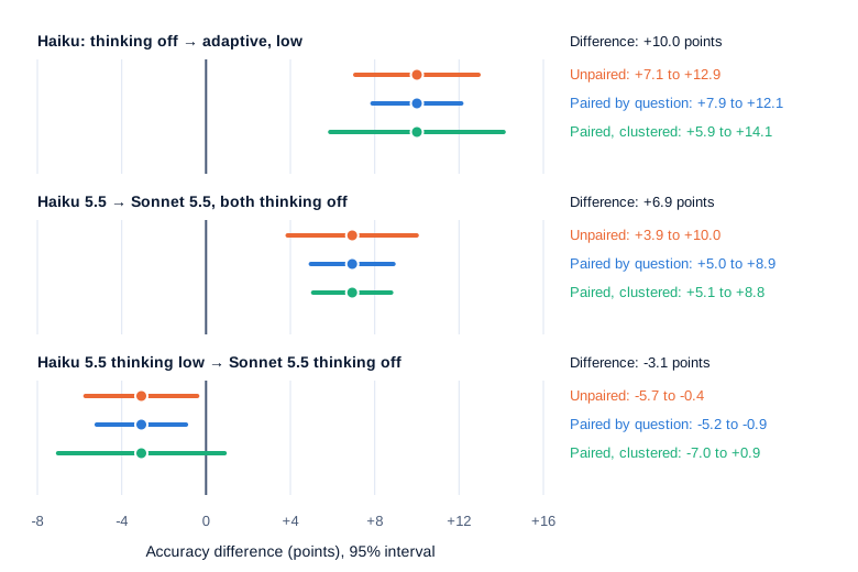
From Scratch Part 9 left paired tests to this series. Take Haiku against Sonnet, both thinking off: Sonnet scored 6.9 points higher. Treated as if they came from separate question sets, the difference has a standard error of sqrt(SE_A² + SE_B²) = sqrt(1.19² + 1.01²) = 1.56 points: a 95% interval of +3.9 to +10.0.
They share questions, though. Pair them, and each question’s difference is +1 (only Sonnet right), -1 (only Haiku right) or 0 (both right or both wrong). The mean of those 1,140 differences has a standard error of 1.00 point, and the interval narrows to +5.0 to +8.9. The gain comes from correlation, ρ: the two models’ results correlate at 0.60 across questions, because a hard question is hard for both. Miller’s SE_paired² = SE_A² + SE_B² - 2 ρ SE_A SE_B gives the same 1.00.
| Both thinking off | Sonnet right | Sonnet wrong |
|---|---|---|
| Haiku right | 881 | 28 |
| Haiku wrong | 107 | 124 |
Only the 135 questions where the two disagree say anything about which is better. McNemar’s test (1947) uses just those: if the models were equally good, each disagreement would be a coin flip, and 107 heads in 135 flips would be very unlikely.
from scipy.stats import binomtest

haiku_only, sonnet_only = 28, 107      # questions only one of the two got right
p = binomtest(sonnet_only, haiku_only + sonnet_only, 0.5).pvalue
print(f"{p:.1e}")                      # 4.4e-12
The p-value, the chance of a split at least this lopsided if there were no real difference, is 4 in a trillion. A paired t-test on the per-question differences gives t = 6.94 and a similar p-value, a paired bootstrap gives +4.9 to +9.0 points, and none of 20,000 random sign flips of the differences produced a gap as large. McNemar’s test is exact for right-or-wrong scores; the t-test and the bootstrap also handle partial credit, averages of several answers and judge scores.
Swipe to pan the diagram, or tap it to zoom.
When the gain sits in a few subjects
Pairing narrowed the interval by 20% to 36% across the three comparisons, while clustering by subject widened two of them. Haiku with a little thinking scored 3.1 points above Sonnet without it. Paired by question, the interval is -5.2 to -0.9 points and McNemar’s test gives p = 0.006 (94 questions to 59): a clear win. Clustered by subject, the interval is -7.0 to +0.9 and includes zero.
The gain is concentrated. High school mathematics alone accounts for 13 of Haiku’s net 35-question lead, and five calculation-heavy subjects (high school and college mathematics, abstract algebra, college physics, professional accounting) together account for 42, more than all of it; on the other subjects, Sonnet was slightly ahead. So “Haiku with thinking beats Sonnet without on these 57 subjects” holds, and “on knowledge questions in general” isn’t shown. The thinking gain sits in the same five subjects, 49 of its net 114 questions, and on 63 of the 138 questions it won, Haiku’s thinking-off reply had been cut off at 16 tokens mid-calculation: a harness effect as much as a reasoning one.
Step 4: how many questions you need
Power and the minimum detectable effect
Statistical power is the chance that an experiment detects a difference that is really there; the usual target is 80%, with a 5% false-alarm rate. The minimum detectable effect (MDE) is the smallest true gap an eval of a given size detects with that power. Miller’s equations 9 and 10 give both from the variance parts measured above:
n = (z_α/2 + z_β)² × (ω² + σ_A²/K_A + σ_B²/K_B) / δ²Here δ is the true gap, ω² the variance of the true per-question differences, σ² each system’s within-question sampling variance and K its answers per question; z_α/2 + z_β is 1.96 + 0.84. Miller’s example, with made-up but “reasonable” values, needs about 969 questions for a 3-point gap, and he concludes that “new evals should contain at least 1,000 questions”.
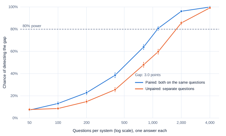
The measured version, for Haiku with thinking low against Sonnet with thinking off: δ = 3.0 points over all answers, ω² = 0.116, σ² = 0.013 and 0.004. With one answer each, n = 7.85 × (0.116 + 0.013 + 0.004) / 0.03² ≈ 1,165 questions. Five answers each would need 1,041 and unlimited answers 1,010. Without pairing, the same gap needs 1,804 questions per system.
Resampling checks the formula. Draw 1,165 questions with replacement from the 1,140, take one recorded answer per system per question, test, and repeat 3,000 times: the paired test found the gap in 79.7% of draws. Unpaired, it found it in 60.4% at that size and in 79.7% at 1,804 questions.
Swipe to pan the diagram, or tap it to zoom.
This 1,140-question eval sits at the edge for a 3-point gap: its MDE is 3.0 points paired and 3.8 unpaired. A 1-point gap with the same variance would need about 10,500 paired questions, three-quarters of MMLU’s test split. The 6.9-point gap between Haiku and Sonnet without thinking needs only 202 paired questions (resampling gave 82.9% power) and 489 unpaired. The support-bot eval post applies the same arithmetic to release gates.
Step 5: many models at once
Twenty copies of one model
A leaderboard compares every model with every other. With 20 models that is 190 pairs, and a test with a 5% false-alarm rate, run 190 times, raises alarms even when every model is identical.
Haiku’s five real runs are five identical “models”: their scores spread over 1.0 point and none of the 10 pairs differed at the 5% level. For a full leaderboard, simulate 20 copies: each answers every question once, right with that question’s measured success rate, and every pair gets an exact McNemar test. Over 1,000 such leaderboards, the gap between the top and bottom copy had a median of 1.0 point and a 95th percentile of 1.3. On average 5.4 of the 190 pairs came out “significant” at p < 0.05, and 82.3% of leaderboards had at least one. That is fewer than the 9.5 a 5% rate implies, because the exact test is conservative when few questions disagree.
Corrections
Three standard corrections set the rule for which p-values to believe:
| Method | Rule | Controls |
|---|---|---|
| Bonferroni | believe p ≤ α / m, for m comparisons | the chance of any false alarm |
| Holm (1979) | sort p-values; believe the j-th smallest while p ≤ α / (m − j + 1) | the same, with more power |
| Benjamini-Hochberg (1995) | believe the k smallest, for the largest k with p ≤ α k / m | the expected share of false alarms among findings |
With Holm’s method, 1.2% of the simulated leaderboards raised any false alarm, and the three real comparisons in Step 3 (largest p-value 0.006) survive every correction. Corrections cost power. With 190 comparisons, Holm’s first threshold is 0.05 / 190, which raises the MDE by a factor of 1.6: 1,140 questions that resolve a 3.0-point gap in one comparison resolve only about 4.9 points on a 20-model leaderboard. Holm suits decisions where any false claim is costly, such as a release gate; Benjamini-Hochberg suits screening many prompt variants, where a few false leads are acceptable.
In the real world
- Meta’s Llama 3 paper (2024) gives its pre-trained models’ scores with “95% confidence intervals (CIs), assuming that benchmark scores are Gaussian distributed”, following Madaan et al. On HumanEval’s 164 problems that gives Llama 3 8B 37.2 ± 7.4 and Llama 3 405B 61.0 ± 7.5, against GPT-4 at 67.0 ± 7.2: a 6-point gap the intervals can’t separate. Reported by Meta, not reproduced here.
- Anthropic’s Claude Haiku 5.5 system card (October 7, 2026) mixes these tools. Terminal-Bench 4.0 errors are computed “with trials treated as independent” (±1.9 points for Haiku 5.5), Terminal-Bench-Science reports a standard error “clustered by task” (±3.7 points), and PhysicianBench gives a 9.4-point lead over another model as “95% confidence interval 2.6 to 16.2 points, paired by task”. Its Global MMLU number, 87.8%, comes from “a single trial”. Reported by Anthropic, not reproduced here.
- Card et al. (2020) found “underpowered experiments are common” in NLP: “typical test sets of 2000 sentences have approximately 75% power to detect differences of 1 BLEU point” in machine translation.
- tinyBenchmarks (Polo et al., 2024) reports that to estimate a model’s MMLU score “it is sufficient to evaluate this LLM on 100 curated examples”; picked at random, 100 questions gave ±7.7 points here. Madaan et al. (2024), measuring scores across ten 7B models that differed only in seed, found that item analysis and item response theory “struggle to meaningfully reduce variance”.
- Miller’s third recommendation, scoring with the probability a model gives the right answer instead of its sampled choice, cuts variance on open models. The Claude API returns no token log-probabilities, so it wasn’t available here.
Common misconceptions
- “Rerunning the eval gives you the error bar.” Five runs spread over 1.0 point, while the error bar from the choice of questions was ±2.3 points, or ±4.2 by subject.
- “If two scores’ error bars overlap, the difference isn’t real.” Haiku with thinking low (87.8% to 91.4%) and Sonnet without thinking (84.6% to 88.5%) overlap, yet the paired test gives p = 0.006, because both saw the same questions.
- “More questions always fix it.” When questions come in groups, the number of groups limits precision: drawn by whole subjects, the naive interval covered the truth about 72% of the time at every size.
- “The bootstrap is always safe.” On 10 questions its “95%” interval covered the truth 86% of the time, against the Wilson interval’s 97%.
- “p < 0.05 on a leaderboard means a real gap.” With 190 comparisons among identical models, 82% of simulated leaderboards had at least one such gap.
Key takeaways
- A score is an estimate from a sample of questions. Report it with a 95% interval and say how many questions it rests on.
- The questions are the unit. Rerunning them measures consistency; only more, and more varied, questions shrink the error bar.
- If questions come in groups, such as subjects or passages, cluster the standard error on the groups. Here that nearly doubled it.
- Compare systems on the same questions and test the per-question differences. Pairing cut the error bar by 20% to 36%, and McNemar’s test fits in four lines.
- Before you run, work out the smallest gap your eval can detect. On 1,140 questions it was about 3 points; on a 20-model leaderboard, about 5.
What’s next
Every number here held the harness fixed: one prompt, one answer format, one rule for reading the reply. Even so, 333 of Haiku’s replies were cut off before reaching a letter, and that limit alone moved the thinking comparison. Part 4 changes the harness and keeps the model: prompt formats, few-shot examples, option order and answer extraction, each measured as a paired difference with the tools from this part.
Further reading
- Adding Error Bars to Evals: A Statistical Approach to Language Model Evaluations (Miller, 2024): the standard, clustered and paired errors and the sample-size formula used throughout.
- A statistical approach to model evaluations (Anthropic, 2024): the five recommendations in short form.
- Position: Don’t Use the CLT in LLM Evals With Fewer Than a Few Hundred Datapoints (Bowyer, Aitchison and Ivanova, 2025): coverage of Wald, bootstrap, Wilson and Bayesian intervals on small evals.
- Quantifying Variance in Evaluation Benchmarks (Madaan et al., 2024): seed variance across training runs, and why item response theory didn’t reduce it.
- With Little Power Comes Great Responsibility (Card et al., 2020): how often NLP comparisons are underpowered.
- Note on the sampling error of the difference between correlated proportions or percentages (McNemar, 1947): the paired test for right-or-wrong outcomes.
- Controlling the False Discovery Rate: A Practical and Powerful Approach to Multiple Testing (Benjamini and Hochberg, 1995): the correction for screening many comparisons.
- Measuring Massive Multitask Language Understanding (Hendrycks et al., 2020): the MMLU benchmark.
- The Llama 3 Herd of Models (Grattafiori et al., 2024): benchmark tables reported with 95% intervals.
- tinyBenchmarks: evaluating LLMs with fewer examples (Polo et al., 2024): estimating scores from 100 curated items.