
Build an LLM From Scratch · Part 3 of 15
The Pretraining Data Pipeline: 2.5 Billion Tokens on a Laptop
Download FineWeb-Edu, check its filters, remove near-duplicates with MinHash, then tokenize, shuffle and pack the series' training data into token shards.
On this page
TL;DR
This part builds the series’ training data and data.py, the module that feeds it to the model. It downloads 2,424,000 FineWeb-Edu documents (11.5 GB of text), checks what FineWeb-Edu’s own filters already removed, and finds 42,867 near-duplicates with MinHash and locality-sensitive hashing, almost all copied between Common Crawl snapshots that FineWeb never compared. The rest is tokenized at 3.3 million tokens per second on 8 CPU cores, shuffled, split off into a 15-million-token validation set, and packed into 2.47 billion training tokens, 1.4 times what the 17-hour run needs. The loader serves them about 10,000 times faster than training reads them.
Why it matters
Part 1’s training run reads 28,296 tokens per second for 17 hours. Every one of those 1.76 billion tokens comes from this pipeline, and mistakes here crash nothing. A duplicated page is simply trained on twice; a validation document that also sits in training makes the held-out loss look better than it is.
One of them shows up as soon as the sample is checked. FineWeb-Edu is already deduplicated, but only within each crawl. Across crawls, 1.8% of the documents downloaded here have a near-copy, like a 2005 Guardian article on heart health republished by another site 17 years later, or the same Wiktionary entry captured on the desktop site in 2017 and the mobile site in 2018.
Fundamentals Part 12 told how labs filter the web into training data. This part does a small version on a laptop, measures each step, and ends with the token shards Parts 5 to 7 train on.
The intuition
Picture a teacher assembling a course reader from a newspaper archive. The archivist has already thrown out the ads, the classifieds and anything not worth teaching, and removed reprints within each year’s volume. But a good article often reappears in a later year, so the teacher compares across years and keeps one copy. Then the teacher shuffles the articles, so a student doesn’t read all of 2017 before reaching 2023, and binds them into volumes of exactly the same thickness, one article after another with a marked break between them. A student can open any volume to any page and keep reading.
The analogy breaks in two places. The teacher judges a reprint by reading it; MinHash only counts how many five-word phrases two pages share, so a rewritten article with the same facts survives and a template page with different names inside it doesn’t. And the student knows where one article ends. The model only sees a single token, id 0, and has to learn from data alone that what follows it is unrelated.
Step 1: what FineWeb-Edu already did, and what we download

The two heavy branches took 7 and 13 minutes on 8 CPU processes; deduplication, the overlap check and packing took about 2 more.
The filters already applied
FineWeb-Edu is FineWeb with one more filter. The FineWeb paper lists every step from raw Common Crawl to the 15-trillion-token dataset, and the FineWeb-Edu dataset card adds the last one:
| Stage | What it does | Threshold or setting |
|---|---|---|
| Text extraction | trafilatura on the raw HTML (WARC files) | instead of Common Crawl’s own text |
| URL filter | Blocklist of adult sites | blocklist match |
| Language ID | fastText classifier | English score at least 0.65 |
| Gopher quality filters | Length, word length, symbols, bullets, stop words | 50 to 100,000 words; mean word length 3 to 10 characters; at least 2 of “the, be, to, of, and, that, have, with” |
| Gopher repetition filters | Repeated lines, paragraphs and n-grams | e.g. duplicate lines at most 30% of lines |
| MinHash dedup, per crawl | 5-word shingles, 112 hashes, 14 bands of 8 | targets 75% similarity |
| C4 filters | Drop lines mentioning javascript or cookie policies; drop pages with “lorem ipsum” or { | all but C4’s terminal-punctuation rule |
| FineWeb custom filters | Drop pages where few lines end in punctuation, many characters sit in duplicated lines, or most lines are short | 0.12, 0.1, 0.67; about 22% of tokens removed |
| PII (personal data) | Email and public IP addresses anonymized | all matches |
| Educational classifier (FineWeb-Edu only) | Scores 0 to 5, rounded to an integer | keep 3 and up; 92% of FineWeb removed |
The Gopher rules come from Table A1 and Appendix A of the Gopher paper. The classifier learned from synthetic labels: Llama-3-70B-Instruct scored 460,000 pages for educational value, focusing on “grade-school and middle-school level knowledge,” and a linear regression head on the Snowflake-arctic-embed-m embedding model learned to predict those scores. At a threshold of 3 it reached an F1 score of 82% against Llama 3’s labels on 50,000 held-out pages. Running it over 15 trillion tokens took 6,000 H100 GPU-hours.
Which 2.4 million documents
FineWeb-Edu’s sample-10BT is a random subset of about 10 billion GPT-2 tokens, published as 14 Parquet files totalling 28.5 GB. Parquet is a column-oriented file format that stores rows in blocks called row groups; here each row group holds 1,000 documents. The run needs 1.76 billion training tokens plus validation and headroom, so a quarter of the sample is enough.
Taking the first three or four files would have been a mistake: each holds only 6 to 12 of the sample’s 95 crawls. Instead, data.download() reads every fourth row group of all 14 files, using HTTP range requests so only those row groups cross the network. (Three whole files were already on disk from that first plan; their row groups were read locally and the files deleted.)
| What | Measured |
|---|---|
| Documents | 2,424,000 from 2,424 row groups |
| Crawls covered | 95, from CC-MAIN-2013-20 to CC-MAIN-2024-10 |
| Text | 11.51 GB of UTF-8 |
GPT-2 tokens (dataset’s token_count column) | 2,496,993,148 |
| On disk, re-compressed with zstd | 4.7 GB |
| Wall time | 614 s with 8 download threads |
The educational scores
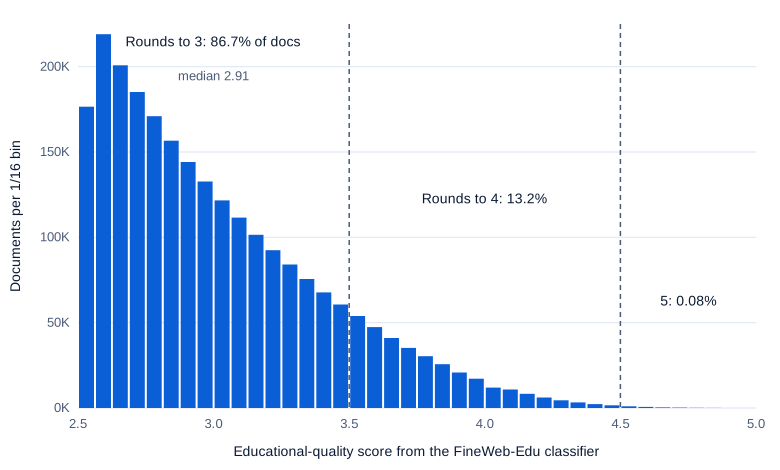
Each document carries the classifier’s raw score and the rounded int_score. “Rounded to 3 or more” means a raw score of at least 2.5, and most documents sit just above that line:
Swipe to pan the diagram, or tap it to zoom.
Half the documents score below 2.91, and only 1,859 of 2.4 million round to 5. Raising the threshold to 3.5 would keep 13% of the documents and 14% of the tokens. The dataset card warns against it too: higher thresholds help knowledge benchmarks but one “significantly degrades performance on HellaSwag and PIQA.” This pipeline keeps the published threshold.
Step 2: one more filter, measured before it’s applied
Very short documents
A common extra rule drops very short documents. They’re the most likely to be fragments, and a 60-token document fills 6% of a 1,024-token context window. Measured with our tokenizer, before deduplication:
| Rule: drop documents under | Documents removed | Share of documents | Share of tokens | Mean edu score of removed |
|---|---|---|---|---|
| 64 tokens | 439 | 0.02% | 0.001% | 2.97 |
| 100 tokens | 17,883 | 0.74% | 0.06% | 2.94 |
| 128 tokens | 52,851 | 2.2% | 0.22% | 2.94 |
| 256 tokens | 353,802 | 14.6% | 2.6% | 2.98 |
The whole sample averages 3.01, so short documents score barely lower. Twelve of them, read by hand, were dictionary entries, a lesson-plan summary and a physics exercise: short, not junk. Gopher’s rule already removed everything under 50 words; the shortest document here has 39 of our tokens.
So the filter stays light: MIN_TOKENS = 64 removes 437 documents after deduplication, 26,599 tokens. It’s a floor for when the pipeline is pointed at less-filtered data.
Part 2’s tokenizer sample
Part 2 trained the tokenizer on the first 800 documents of each FineWeb-Edu crawl. FineWeb-Edu has roughly 1.3 billion documents (1.3 trillion tokens at about 1,000 per document). If both samples were independent random draws, about 170 of our 2.4 million documents would also be among those 88,000. Hashing the text found 2,010 exact matches, 12 times more, so the two samples are clearly not independent. With near-duplicates (same LSH cluster, see Step 3) it’s 3,850.
That’s harmless for training, but validation should be text no part of the pipeline has seen, so these 3,850 documents can only land in training.
Step 3: near-duplicates with MinHash and LSH
Shingles and Jaccard similarity
Two documents are compared as sets. A shingle is a run of n consecutive words; data.py lowercases the text, splits it into words and takes every 5-word shingle, as FineWeb does. The Jaccard similarity of two sets is the size of their intersection divided by the size of their union: 1 for identical sets, 0 for nothing in common.
Two nine-word sentences that differ in their last word:
import numpy as np
from data import shingles, minhash
a = "the cat sat on the mat and then slept"
b = "the cat sat on the mat and then left"
sa, sb = shingles(a), shingles(b)
print(len(np.intersect1d(sa, sb)) / len(np.union1d(sa, sb)))   # 0.6666666666666666
print((minhash(a) == minhash(b)).mean())                        # 0.7410714285714286
Each sentence has 5 shingles; 4 are shared and the union holds 6, a similarity of 4/6. One changed word drops it to 0.67 because that word sits in five shingles. In a thousand-word document, a few edits barely move it.
MinHash: a short signature that estimates similarity
Comparing 2.4 million documents in pairs means 2.9 trillion comparisons. MinHash avoids that. Hash every shingle with a hash function and keep only the smallest value. For two documents, the smallest hash over their union belongs to one shingle; the two minimums are equal exactly when that shingle is in both sets. So the chance that the minimums match is the Jaccard similarity, as the Mining of Massive Datasets lecture notes on locality-sensitive hashing prove.
Do this with 112 different hash functions and you get a 112-number signature per document. The fraction of positions where two signatures agree estimates their similarity, with a standard error of about sqrt(s(1 - s)/112), 0.04 at s = 0.75. The sentences above have true similarity 0.667 and signature agreement 0.741, 1.7 standard errors off; with only 6 shingles in the union, that’s ordinary noise.
# data.py (excerpt)
SEEDS = np.random.default_rng(42).integers(0, 2**63, N_HASH, dtype=np.uint64)  # one per hash function

def mix64(x):
    """MurmurHash3's 64-bit finalizer: scrambles every input bit into every output bit."""
    x = x ^ (x >> np.uint64(33))
    x = x * np.uint64(0xFF51AFD7ED558CCD)                # uint64 arithmetic wraps around mod 2^64
    x = x ^ (x >> np.uint64(33))
    x = x * np.uint64(0xC4CEB9FE1A85EC53)
    return x ^ (x >> np.uint64(33))

def minhash(text):
    """112 MinHash values: for each hash function, the minimum over the document's shingles."""
    x = shingles(text)
    sig = np.full(N_HASH, np.iinfo(np.uint64).max, dtype=np.uint64)
    for s in range(0, len(x), 2048):                     # blocks keep memory flat on huge docs
        h = mix64(x[None, s:s + 2048] ^ SEEDS[:, None])  # hash function i: mix64(shingle XOR seed_i)
        sig = np.minimum(sig, h.min(axis=1))
    return (sig >> np.uint64(32)).astype(np.uint32)       # keep the top 32 bits
Stored as 32-bit numbers, a signature is 448 bytes; the sample’s take 1.09 GB.
Bands and rows: turning signatures into buckets
Comparing all pairs of signatures is still too slow. Locality-sensitive hashing (LSH) splits each signature into b bands of r rows and puts two documents in the same bucket if all r values of any one band match. FineWeb uses 14 bands of 8.
For two documents with similarity s, one band matches with probability s^8. All 14 miss with probability (1 - s^8)^14, so they’re flagged with probability 1 - (1 - s^8)^14. At s = 0.5 that’s 5%; at 0.75, 77%; at 0.8, 92%; at 0.9, essentially 100%. The curve is an S whose steepest point sits near (1/b)^(1/r) = (1/14)^(1/8) = 0.72, which is how the band shape sets the similarity threshold.
In code, each band becomes a 32-byte key, the keys are sorted, and equal neighbours are candidate pairs:
# data.py (excerpt)
def lsh_pairs(sigs):
    """Candidate duplicate pairs: documents whose 8 values agree in at least one of the 14 bands."""
    pairs = []
    for b in range(BANDS):
        band = np.ascontiguousarray(sigs[:, b * ROWS:(b + 1) * ROWS])
        keys = band.view(np.dtype((np.void, band.dtype.itemsize * ROWS))).ravel()
        order = np.argsort(keys, kind="stable")
        same = keys[order][1:] == keys[order][:-1]           # neighbours in sorted order collide
        pairs.append(np.stack([order[:-1][same], order[1:][same]], axis=1))
    return np.unique(np.concatenate(pairs), axis=0)
Pairs are then joined into clusters with union-find, a structure that tracks which items are connected, so if A matches B and B matches C, all three are one cluster even when A and C share no band. One randomly chosen document per cluster is kept, FineWeb’s rule.
Checking the curve, and a bug it caught
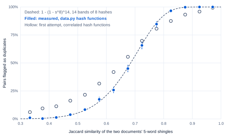
The S-curve can be measured. scurve.py took 600 held-out documents, made 20 copies of each with a random 0 to 12% of the words replaced, and checked whether LSH flagged each of the 12,000 pairs, binned by exact 5-gram similarity:
Swipe to pan the diagram, or tap it to zoom.
With the final hash functions every bin matches the formula within its 95% interval: 26% flagged at similarity 0.63 against 28% predicted, 85% at 0.78 against 85%.
The first version didn’t. It used the textbook universal hash h(x) = (a·x + b) mod p with p = 2^61 - 1, but drew a, b and the shingle hash x below 2^32 to avoid 64-bit overflow. Then a·x wraps around p at most 8 times, so every hash function orders the shingles almost the same way and picks nearly the same minimum: the 112 hashes were correlated. Signature agreement missed the true similarity by 0.13 to 0.16 instead of 0.03 to 0.04, and pairs at 0.33 similarity were flagged 6.1% of the time instead of 0.2%. Nothing crashed, so only the measured curve showed it. A strong 64-bit mixer, MurmurHash3’s finalizer, fixed it.
What deduplication found
MinHash signatures for all 2,424,000 documents took 421 s on 8 processes (2,800 CPU-seconds, about 4 MB/s per core); LSH and clustering took 16 s more.
| Result | Count |
|---|---|
| Candidate pairs | 43,211 |
| Duplicate clusters | 41,459 |
| … of 2 documents | 40,545 |
| … spanning two or more crawls | 41,394 (99.8%) |
| … whose texts are byte-for-byte identical | 25,989 (63%) |
| Documents removed | 42,867 (1.77%) |
| Tokens removed | 47,635,678 (1.88%) |
| Pairs whose signatures agree on under half the values | 411 (1.0%) |
That’s what FineWeb’s design predicts: each crawl was deduplicated on its own, so what’s left are copies between crawls. Only 65 clusters sit inside one crawl.
A few of the pairs, with their exact 5-gram similarity:
- A 2005 Guardian article on heart health (CC-MAIN-2016-07) and “Top 10 Tips for Healthy Heart” on quiet-corner.com (CC-MAIN-2022-33): 0.79. The second adds an introduction, then repeats the list (“1. Stop smoking. Quitting smoking is the single most important thing…”).
- Wiktionary’s entry for “noun”, desktop site in CC-MAIN-2017-04 and mobile site in CC-MAIN-2018-05: 0.93. The desktop page adds a table of contents (“1 English, 2 Chuukese, 3 Occitan…”).
- Enchanted Learning’s tsunami page (CC-MAIN-2014-23) and a copy on a tripod.com student page (CC-MAIN-2018-34): 0.77. Both say “Tsunamis are caused by an underwater earthquake, a volcanic eruption, an sub-marine rockslide,” typo included.
The largest cluster has 148 documents: Ancestry.com family-tree pages from crawls between 2016 and 2018, one per surname, each starting “Find more Grzechowiak relatives and grow your tree by exploring billions of historical records.” Only the surname changes. FineWeb’s authors credit most of deduplication’s benefit to removing template clusters like this, which at full scale hold hundreds of thousands of documents.
Does removing 1.8% help accuracy? Probably not much: the card reports that deduplicating FineWeb-Edu “doesn’t have any impact on model performance” for a 1.8B model trained on 350B tokens. The case here is the validation set. A validation document with a near-copy in training measures memory, not generalization, and with every cluster cut to one document before the split, none has a near-copy LSH can find.
Step 4: tokenize, shuffle and pack
Tokenizing 11.5 GB
Each document is encoded with Part 2’s 32,768-token tokenizer and followed by <|endoftext|>, id 0. With encode_special_tokens = True, the one document in the sample that contains the literal text <|endoftext|> gets it spelled out as ordinary tokens instead of a fake document boundary:
# data.py (excerpt)
def encode_docs(tok, texts):
    """Token ids for a batch of documents, each followed by <|endoftext|> (id 0)."""
    return [enc.ids + [EOT] for enc in tok.encode_batch_fast(texts)]
encode_docs(encoder(), ["The cat sat."]) returns [[469, 2289, 2472, 21, 0]]. Throughput, measured on Part 2’s 26 MB held-out set and then on the full run:
| Setup | Text throughput | Tokens per second |
|---|---|---|
| 1 process, 1 thread (held-out set) | 2.96 MB/s | 643,000 |
1 process, 8 threads, encode_batch_fast (held-out set) | 10.8 MB/s | 2.35 million |
| 8 processes, 1 thread each (full 11.5 GB) | 14.9 MB/s | 3.28 million |
The full run took 772 s with other jobs sharing the machine. At that rate the 1.76 billion training tokens take 9 minutes to produce and 17 hours to train on.
The sample comes to 2,531,814,962 tokens including the 2,424,000 end-of-text markers: 4.55 bytes of text per token. Part 2 measured 4.61 on its held-out set. The gap is the text, not the tokenizer: on the same two samples, GPT-2’s counts move from 4.66 to 4.61 bytes per token, and ours stays 1.1 to 1.3% behind GPT-2’s on both.
Shuffling and the validation split
After deduplication and the length floor, 2,380,696 documents remain. A seeded permutation (seed 1337) shuffles them as whole documents. The first ones in that order, skipping the 3,850 that overlap Part 2’s sample, become validation until it holds 15 million tokens; the rest become training, in the same shuffled order:
| Split | Documents | Tokens | Files |
|---|---|---|---|
| Validation | 14,561 | 15,001,119 | val_000.bin (30 MB) |
| Training | 2,366,135 | 2,469,151,566 | train_000.bin to train_024.bin (4.94 GB) |
Training has 1.40 times the 1,761,607,680 tokens Part 7 needs, so the main run never repeats a token, and the leftover 707 million can extend a run or feed Part 8’s scaling sweep. The pack step took 80 s.
Because documents are shuffled before packing, the loader can read the shards in order: consecutive windows come from unrelated documents and crawls.
The shard format
Each shard is a flat file: a 1,024-byte header of 256 32-bit integers (a magic number, a version and the token count, the same layout as llm.c’s .bin files), followed by up to 100 million tokens as uint16. With 32,768 tokens in the vocabulary every id fits in two bytes, so 100 million tokens take 200 MB. NumPy’s memmap maps the file into memory without reading it; the operating system loads pages only when they’re touched.
Packing versus padding
In the training split the median document is 627 tokens and the mean 1,043; 27% are longer than the 1,024-token context and hold 65% of the tokens. There are two ways to make fixed-size rows from them.
Padding gives each document its own rows: a long document is cut into 1,024-token rows and the last row of every document is filled with a dummy token the loss ignores. On this data that’s 3,693,256 rows, and 34.7% of their positions are padding. The GPU would spend about a third of its time on nothing, stretching the 17.3-hour run to about 26.5 hours.
Packing concatenates every document and its id 0 into one stream and cuts the stream into windows of 1,024. Nothing is wasted. The cost is that windows mix documents: 61% of windows contain at least one document boundary, a window holds 1.98 documents on average, and 37.5% of training tokens sit in a window after the end of an earlier, unrelated document.
Cross-document attention
With causal attention, those 37.5% of tokens can attend to the unrelated text before them. Two fixes exist. Document masking blocks attention across id 0, so each token sees only its own document; Llama 3 does this but reports the change “had limited impact during in standard pre-training” and mattered mainly “in continued pre-training on very long sequences.” The other option is to do nothing, as GPT-3 did: documents “are not masked in any special way” and are only “delimited with a special end of text token.”
This series does what GPT-3 did. A mask needs per-window bookkeeping and an attention kernel that accepts it, for a gain Llama 3 found small even at its scale. Id 0 marks every boundary, so the model can learn that the text after it starts fresh.
Step 5: a loader that never makes the GPU wait
The training loop in Part 5 asks for micro-batches of 16 sequences of 1,024 tokens, 32 of them per optimizer step. ShardLoader treats all train shards as one stream and defines micro-batch i as the window that starts at token i × 16 × 1,024:
# data.py (excerpt)
class ShardLoader:
    """(x, y) micro-batches of B sequences of T tokens, read straight from the shards.

    The shards are one long token stream; micro-batch i is the window starting at token i*B*T,
    so batch(i) is a pure function of i: deterministic, and resumable from any step.
    """

    def __init__(self, split="train", B=16, T=1024, data_dir=SHARD_DIR):
        self.B, self.T = B, T
        self.shards = [read_shard(p) for p in sorted(glob.glob(os.path.join(data_dir, f"{split}_*.bin")))]
        self.ends = np.cumsum([len(s) for s in self.shards])
        self.n_tokens = int(self.ends[-1])
        self.n_batches = (self.n_tokens - 1) // (B * T)

    def window(self, start, n):
        """n tokens of the stream from `start`, stitched across a shard boundary if needed."""
        out, k = [], int(np.searchsorted(self.ends, start, side="right"))
        offset = start - (self.ends[k - 1] if k else 0)
        while n > 0:
            piece = self.shards[k][offset:offset + n]
            out.append(piece)
            n, k, offset = n - len(piece), k + 1, 0
        return np.concatenate(out) if len(out) > 1 else out[0]

    def batch(self, i):
        import torch
        BT = self.B * self.T
        buf = torch.from_numpy(self.window((i % self.n_batches) * BT, BT + 1).astype(np.int64))
        return buf[:-1].view(self.B, self.T), buf[1:].view(self.B, self.T)

    def batches(self, step=0, accum=32):
        """Micro-batches from optimizer step `step` on (accum micro-batches per step)."""
        i = step * accum
        while True:
            yield self.batch(i)
            i += 1
The targets y are the inputs x shifted by one token: reading 16,385 tokens and slicing gives both. Resuming after a crash needs only the step number:
from data import ShardLoader
loader = ShardLoader("train", B=16, T=1024)
batches = loader.batches(step=1200)          # resume at optimizer step 1,200
x, y = next(batches)
print(x.shape, x.dtype, loader.n_tokens)     # torch.Size([16, 1024]) torch.int64 2469151566
print(bool((x[:, 1:] == y[:, :-1]).all()))   # True
A fresh loader started at step 2,000 returned exactly the same tensors as one that iterated there, and the last micro-batch of the 3,360-step run ends at token 1,761,607,680 of 2,469,151,566.
Throughput, timed over 320 micro-batches (10 optimizer steps) starting at four different steps:
| Measurement | Tokens per second | Times what training needs |
|---|---|---|
| CPU tensors, shards in the page cache | 284 to 340 million | 10,000 to 12,000 |
| Plus pinned copy to the RTX 4060 Laptop GPU, after the first 10 steps (CUDA start-up) | 160 to 209 million | 5,700 to 7,400 |
Reading a shard from disk, bypassing the cache (dd) | 1.2 billion (2.4 GB/s) | 42,000 |
The page cache is the operating system’s copy of recently read files in RAM; even without it, the disk is 42,000 times faster than training. Each micro-batch takes about 0.58 s to train on and under 0.1 ms to load, so prefetching in a background thread would buy nothing measurable.
In the real world
- llm.c’s FineWeb script is the closest relative: GPT-2 tokens in 100-million-token
uint16shards with the same 256-integer header, an end-of-text token before every document, and the first shard used as validation. Its data loader can shuffle the order of shards and of samples inside each one; ours shuffles documents once, at pack time. - nanoGPT keeps all tokens in one
train.binmemmap and draws random offsets withtorch.randintfor every batch, so replaying batches after a crash needs the random generator’s saved state. - FineWeb tried the opposite of per-crawl deduplication. Deduplicating all 96 crawls together left 4 trillion tokens instead of 20 trillion and removed up to 90% of the oldest crawls, and for one 2013 crawl the 10% that survived was worse than what was removed. The paper’s Appendix E also compares FineWeb’s 112 hashes with RefinedWeb’s 9,000 (450 bands of 20) for a sharper cut-off at more compute.
- Lee et al. (2021) found that models trained on deduplicated data “emit memorized text ten times less frequently,” and that train-test overlap “affects over 4% of the validation set of standard datasets.”
- With several GPUs the loader also splits the stream: llm.c’s takes a
process_rankandnum_processesso each GPU reads its own part. Bigger vocabularies outgrowuint16; llm.c stores Llama 3’s 128,256-token ids asuint32.
Common misconceptions
- “FineWeb-Edu is already deduplicated.” Only within each crawl. Across crawls, 1.77% of the documents in our sample had a near-copy, and 99.8% of the duplicate clusters spanned two or more crawls.
- “More filtering is always safer.” A 256-token floor would remove 14.6% of the documents and 2.6% of the tokens, and the short documents scored 2.98 on the educational scale against 3.01 overall. Measure what a filter removes before trusting its name.
- “Padding is the simple, safe choice.” On this data it wastes 34.7% of every batch, about 9 extra hours on the main run. Packing wastes nothing and costs only some cross-document attention.
- “Random hash parameters give independent hash functions.” Our first
(a·x + b) mod pfamily, with smallaandx, produced correlated hashes and a visibly wrong S-curve. Measuring the curve against the formula is a cheap test. - “The data loader is a bottleneck.” For one GPU training a small model it’s 10,000 times faster than needed. The expensive part is the one-time pipeline: 32 minutes of CPU work for 17 hours of GPU work.
Key takeaways
- FineWeb-Edu arrives filtered by URL, language, Gopher and C4-style rules, per-crawl MinHash and an educational classifier that removed 92% of FineWeb. Most kept documents score just above the 2.5 cut-off.
- Sample across the whole dataset, not its first files: each
sample-10BTfile holds only 6 to 12 of the 95 crawls. - MinHash turns a document into 112 numbers whose agreement estimates Jaccard similarity; 14 bands of 8 flag pairs with probability
1 - (1 - s^8)^14. Measuring that curve caught a broken hash family. - Cross-crawl near-duplicates were 1.77% of documents and 1.88% of tokens. Removing them before splitting keeps validation clean.
- The series’ data is 2.47 billion training tokens in 25
uint16shards plus 15 million validation tokens, packed with id 0 between documents. Packing avoids 34.7% padding, and the loader serves batches 10,000 times faster than training consumes them.
What’s next
The data is ready; nothing yet can learn from it. Part 4 writes the model: RMSNorm, rotary position embeddings, grouped-query attention and SwiGLU in under 200 lines of PyTorch, with its parameter count checked against the 88,096,512 from Part 1 and its logits checked against Hugging Face’s Llama.
Further reading
- The FineWeb Datasets: Decanting the Web for the Finest Text Data at Scale (Penedo et al., 2024): every filter, the per-crawl MinHash settings and the global-deduplication experiment.
- FineWeb-Edu dataset card (Hugging Face): the educational classifier, its threshold, the samples and the license.
- Scaling Language Models: Methods, Analysis & Insights from Training Gopher (Rae et al., 2021): Appendix A’s quality and repetition filters, used by FineWeb.
- Deduplicating Training Data Makes Language Models Better (Lee et al., 2021): what duplicates do to memorization and to evaluation.
- Mining of Massive Datasets, Chapter 3 (Leskovec, Rajaraman and Ullman): shingling, MinHash and the banding analysis behind the S-curve.
- Language Models are Few-Shot Learners (Brown et al., 2020) and The Llama 3 Herd of Models (2024): packing with an end-of-text token, and document masking.
- llm.c
fineweb.pyanddataloader.h(Karpathy): a compact reference for token shards and a shard loader.