
Build an LLM From Scratch · Part 1 of 15
Build an LLM From Scratch: What a Laptop Can Train
Measured training speed on an 8 GB laptop GPU, 6ND budget math, and the model this series builds: 88M parameters, 1.76B tokens, about 17 hours.
On this page
TL;DR
This series builds one small GPT-style language model from nothing: tokenizer, data, model, training, evaluation and fine-tuning, all on a laptop with an 8 GB GPU. Before writing any of it, this part measures what the laptop can actually train. A throwaway prototype at four sizes, from 22 to 126 million parameters, trains at 19,000 to 104,000 tokens per second, using 66% to 73% of the GPU’s measured peak. Plugged into the 6ND compute rule and Chinchilla’s 20 tokens per parameter, those rates pick the series’ model: 88 million parameters trained on 1.76 billion tokens in about 17 hours, for about 16 cents of electricity at the GPU.
Why it matters
In 2024, Andrej Karpathy reproduced GPT-2’s smallest model in about 90 minutes on eight A100 GPUs, for about $20 of rented compute. The same 10 billion tokens on a laptop’s RTX 4060 would take about six days.
A laptop can still train a smaller model properly, to the point that scaling-law research calls compute-optimal, in under a day. Choosing that model takes three measured numbers: how many tokens per second the GPU trains at each model size, how much memory each size needs, and how many tokens each size deserves. Get them wrong and you find out 20 hours into a run that it needs 40 more, or that it never fit in memory.
Math Part 15 derived the arithmetic, and Fundamentals Part 12 told the story of scaling laws at data-center size. This part runs that arithmetic against one real machine and fixes the design that the other 14 parts build on.
The intuition
Think of mowing a square lawn. The model’s parameter count is the length of one side. Make the side twice as long and you have twice as many rows to mow, and each row is twice as long. The job takes four times as long.
Training works the same way. A model with twice the parameters costs twice as much compute per token, and the compute-optimal recipe says it should also see twice as many tokens. So the run takes four times as long. That square is why a laptop’s choices are so narrow: going from a one-night model to a one-weekend model only buys about 2.4 times the parameters.
The analogy breaks in two places. A GPU doesn’t mow every size at the same speed: small models leave it partly idle, and too-large batches stop fitting in memory, so the speed has to be measured. And “twice the tokens” is a convention that labs often ignore: many small models today are trained on hundreds of times more tokens than the recipe says, because they’re cheap to run afterward.
Step 1: the decisions fixed for the whole series
Every later part depends on a handful of choices. They’re fixed here so that a tokenizer trained in Part 2 still fits the model in Part 4 and the checkpoint from Part 7 still loads in Part 12.
| Decision | Choice | Why |
|---|---|---|
| Architecture | Decoder-only, Llama-style: RMSNorm, RoPE, grouped-query attention, SwiGLU, tied embeddings | The design nearly every open model now uses (Fundamentals Part 10) |
| Vocabulary | Byte-level BPE, 32,768 tokens | Keeps the embedding table under 30% of a small model; token IDs fit in 2 bytes |
| Context length | 1,024 tokens | Attention stays about 15% of the compute |
| Precision | BF16 mixed precision, FP32 master weights | Tensor cores run BF16; FP32 copies keep small updates from vanishing |
| Batch | 524,288 tokens per optimizer step (512 sequences) | The batch GPT-3 Small and llm.c used for 125M models |
| Optimizer | AdamW (fused) | The standard for LLM pretraining |
| Main data | A sample of FineWeb-Edu | Filtered for educational value; open license |
| Quick-run data | TinyStories | Small models learn it in minutes |
A decoder-only model reads text left to right and predicts the next token, with no separate encoder. RMSNorm (root-mean-square normalization) rescales each token’s vector to a steady size before each sub-layer. RoPE (rotary position embedding) tells attention where each token sits by rotating its queries and keys. Grouped-query attention (GQA) lets several query heads share one key head and one value head, which shrinks the cache used in generation. SwiGLU is the gated feed-forward layer that replaced the older two-matrix MLP. Tied embeddings means one table does two jobs: it turns token IDs into vectors at the input and turns the final vectors back into scores over the vocabulary at the output. Fundamentals Part 10 builds each of these, and Part 4 writes them in code.
The vocabulary size also sets costs. A tokenizer splits text into tokens, the units the model reads; byte-level BPE (byte-pair encoding) starts from the 256 possible bytes and repeatedly merges the most frequent pair (Fundamentals Part 2). With 32,768 tokens and a 768-number vector per token, the shared table holds 25.2 million parameters, 29% of the model chosen below. GPT-2’s 50,257-token vocabulary would push that share to 38%. And since 32,768 is 2 to the 15th, every token ID fits in a 16-bit integer, so 1.76 billion training tokens take 3.5 GB on disk. Part 2 trains the tokenizer and measures how well this size compresses text.
Mixed precision means the matrix multiplications run in BF16 (bfloat16, a 16-bit float with FP32’s range but fewer digits), while the optimizer keeps a full FP32 (32-bit) copy of every weight. In PyTorch that’s torch.autocast with FP32 parameters, and it’s what GPU Part 6’s tensor cores are built for.
FineWeb-Edu is Hugging Face’s filtered web text: pages from Common Crawl that a classifier, trained on ratings from Llama-3-70B-Instruct, scored at least 3 out of 5 for educational value. The dataset card gives 1.3 trillion tokens in all and a sample-10BT subset of about 10 billion GPT-2 tokens, which is where this series draws from. It’s released under the Open Data Commons Attribution License (ODC-By) v1.0, and the card adds that use is also “subject to CommonCrawl’s Terms of Use.” TinyStories is 2.1 million short stories that GPT-3.5 and GPT-4 wrote using only a small vocabulary, under the CDLA-Sharing-1.0 license. Its paper shows that models “below 10 million total parameters” trained on it “still produce fluent and consistent stories,” which makes it the right data for a first run that has to finish in minutes.
Step 2: measuring the laptop
Four candidate models
The prototype is about 60 lines of PyTorch model code in a scratch folder, built only to be timed; Part 4 writes the real model. It uses the decisions above with a head size of 64 and three query heads per key-value head, at four sizes:
| Name | Width d | Layers | Query / KV heads | SwiGLU width | Non-embedding | Embedding | Total |
|---|---|---|---|---|---|---|---|
| 22M | 384 | 6 | 6 / 2 | 1,024 | 9,442,176 | 12,582,912 | 22,025,088 |
| 47M | 576 | 8 | 9 / 3 | 1,536 | 28,321,344 | 18,874,368 | 47,195,712 |
| 88M | 768 | 10 | 12 / 4 | 2,048 | 62,930,688 | 25,165,824 | 88,096,512 |
| 126M | 768 | 16 | 12 / 4 | 2,048 | 100,688,640 | 25,165,824 | 125,854,464 |
The SwiGLU widths are about 8/3 times d, rounded up to a multiple of 256, which gives the MLP’s three matrices about the same parameter count as a classic two-matrix MLP of width 4d. The 126M model is GPT-2 small’s width, with a smaller vocabulary and four more layers.
How the speed was measured
The machine is an NVIDIA GeForce RTX 4060 Laptop GPU (8 GB, 24 SMs) under WSL2, driver 592.82, PyTorch 2.11.0 with CUDA 12.8 and Triton 3.6.0. Each run compiles the model with torch.compile, uses PyTorch’s scaled dot-product attention (which picked the FlashAttention kernel here, grouped-query heads included), BF16 autocast and fused AdamW, and feeds random token IDs with seed 1337. Throughput doesn’t depend on what the tokens say, and the loss stays near ln(32,768) ≈ 10.40, as it should for text with nothing to learn.
A training step here means one AdamW update on 524,288 tokens. The GPU can’t hold 512 sequences at once, so each step runs several micro-batches, small groups of sequences processed together, and adds up their gradients before updating. That’s gradient accumulation: 16 sequences at a time, accumulated 32 times, gives the same update as 512 at once. Each step was timed on the wall clock with torch.cuda.synchronize() on both sides, after a warm-up of two micro-batches, which triggers compilation, and one optimizer update. nvidia-smi logged the SM clock, memory clock, power draw and power limit every second.
How big a micro-batch fits
This table times forward plus backward passes alone, the median of 12 after warm-up, with the peak memory PyTorch allocated:
| Micro-batch (sequences of 1,024) | 22M: tokens/s (peak GiB) | 47M | 88M | 126M |
|---|---|---|---|---|
| 4 | 97,000 (0.99) | 44,800 (1.76) | 26,700 (2.90) | 19,300 (4.19) |
| 8 | 102,600 (1.56) | 45,600 (2.66) | 27,100 (4.21) | 20,300 (6.13) |
| 16 | 102,400 (2.71) | 47,000 (4.43) | 27,000 (6.84) | 2,300 (10.03) |
| 32 | 96,400 (5.00) | 7,900 (8.00) | 2,500 (12.11) | 1,300 (17.83) |
Below the memory limit, the micro-batch barely matters: going from 4 to 16 sequences changes throughput by 6% or less, because even 4 sequences of 1,024 tokens give the matrix multiplications 4,096 rows of work. Above the limit, nothing crashed. PyTorch reported 10 to 18 GiB allocated on a card with 8 GiB, so the overflow went to the laptop’s system memory, and training ran 6 to 16 times slower. At 64 sequences the process was finally killed when its system memory passed the 4 GB cap these experiments run under. A run that silently spills looks healthy in every log except tokens per second, so the series watches that number from the first step.
The largest micro-batch that stays in GPU memory is 32 sequences for the 22M model, 16 for the 47M and 88M, and 8 for the 126M.
Throughput and MFU
MFU (model FLOPs utilization) is the share of the GPU’s peak arithmetic rate spent on the model’s own math. It needs a FLOP count per token, and this series uses the one in Appendix B of the PaLM paper, which nanoGPT’s MFU estimate also uses:
FLOPs per training token = 6N + 12·L·H·Q·THere N is the parameter count, L the layers, H the query heads, Q the head size and T the sequence length. The 6N part is Math Part 15’s rule. The second term is attention’s own matrix multiplications, which use no weights; PaLM says they “add 6LH(2QT) FLOPs per token.” With H·Q = d, it’s 12·L·d·T. For the 88M model that’s 528.6 million FLOPs for the weights plus 94.4 million for attention, 622.95 million per token, with attention at 15%. At a 2,048-token context it would be 26%. PaLM counts the full attention square, so it charges for the masked half that a causal model never needs; Kaplan et al.’s count halves the attention term, and the table shows MFU without attention too.
The peak is GPU Part 4’s measured BF16 roof, 25.3 TFLOPS. Here are full optimizer steps at the largest micro-batch that fits, about 2.5 to 3 minutes per size:
| Model | Micro-batch × steps accumulated | Seconds per step | Tokens/s | TFLOPS (PaLM count) | MFU | MFU, 6N only | SM clock, median (range) | GPU power, mean | Power limit |
|---|---|---|---|---|---|---|---|---|---|
| 22M | 32 × 16 | 5.06 | 103,618 | 16.6 | 65.7% | 54.1% | 1,920 (1,695-2,055) MHz | 49.9 W | 49-50 W |
| 47M | 16 × 32 | 10.60 | 49,459 | 16.8 | 66.4% | 55.4% | 1,935 (1,695-2,010) MHz | 49.8 W | 48-50 W |
| 88M | 16 × 32 | 17.77 | 29,508 | 18.4 | 72.7% | 61.7% | 1,920 (1,650-1,995) MHz | 49.5 W | 45-50 W |
| 126M | 8 × 64 | 27.46 | 19,096 | 17.3 | 68.4% | 57.0% | 1,830 (1,605-2,025) MHz | 46.0 W | 43-50 W |
These runs took 30, 14, 9 and 7 steps. The memory clock held 7,000 MHz, the GPU warmed from 65 to 82 °C, and the only throttle reason nvidia-smi reported was the software power cap. Steps within a run varied by about 4% at most.
Seventy percent of peak is high; llm.c describes itself as “quite efficient at up to ~60% model flops utilization” on A100s. Part of the gap is the yardstick. GPU Part 4 measured 25.3 TFLOPS with the SM clock at 2,175 MHz, and during these runs it sat near 1,900. Against the 29.1 TFLOPS the spec sheet implies at the 2,370 MHz boost clock, the 88M model’s 18.4 TFLOPS is 63%. MFU against a laptop’s measured roof is a fair way to compare model sizes on one machine, and a poor way to compare machines.
Sustained speed
The real run lasts hours. Over 10 minutes (32 steps, 593 seconds), the 88M model settled at 28,296 tokens per second, 4% below its short run. The power limit wandered between 39.6 and 49.7 W, power averaged 46.1 W, the SM clock’s median fell to 1,815 MHz, the GPU reached 83 °C, and the memory clock dipped once to 5,870 MHz. That’s 69.7% MFU on the PaLM count. The budget below uses the short runs for all four sizes, so they compare fairly, and the sustained figure for the final plan.
Step 3: the budget math
Hoffmann et al. (2022), the Chinchilla paper, found that “for every doubling of model size the number of training tokens should also be doubled”; their Table 3 comes to about 20 tokens per parameter, such as 8.0 billion tokens for a 400-million-parameter model. They count embedding parameters in the total, so this series does too. With D = 20N tokens, the compute is C = 6ND, and the measured tokens per second turn it into hours. The script below is the whole budget:
# Measured on the RTX 4060 Laptop GPU: parameters, tokens/s, mean GPU power in watts
runs = {
    "22M":  (22_025_088, 103_618, 49.9),
    "47M":  (47_195_712,  49_459, 49.8),
    "88M":  (88_096_512,  29_508, 49.5),
    "126M": (125_854_464, 19_096, 46.0),
}
PRICE = 0.20  # illustrative electricity price, $ per kWh

for name, (N, tok_s, watts) in runs.items():
    D = 20 * N                        # Chinchilla: about 20 tokens per parameter
    C = 6 * N * D                     # training FLOPs, 6ND
    hours = D / tok_s / 3600
    kwh = watts * hours / 1000
    night = tok_s * 8 * 3600 / N      # tokens per parameter reachable in 8 h
    weekend = tok_s * 48 * 3600 / N
    print(f"{name:>4}: D={D/1e9:.2f}B  C={C:.1e}  {hours:4.1f} h  "
          f"{kwh:.2f} kWh ${kwh * PRICE:.2f}  night {night:3.0f}/param  weekend {weekend:4.0f}/param")
22M: D=0.44B C=5.8e+16 1.2 h 0.06 kWh $0.01 night 135/param weekend 813/param
47M: D=0.94B C=2.7e+17 5.3 h 0.26 kWh $0.05 night 30/param weekend 181/param
88M: D=1.76B C=9.3e+17 16.6 h 0.82 kWh $0.16 night 10/param weekend 58/param
126M: D=2.52B C=1.9e+18 36.6 h 1.68 kWh $0.34 night 4/param weekend 26/param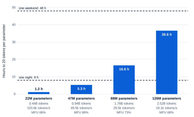
Swipe to pan the diagram, or tap it to zoom.
The square from the lawn shows up in the hours. The 126M model has 5.7 times the parameters of the 22M model and takes 31 times as long.
Read the “night” column the other way, too. Eight hours buys the 22M model 135 tokens per parameter, far past Chinchilla, but gives the 126M model only 4, too few for its size. Since time grows with the square of the size, one night’s compute-optimal model is about 55 to 60 million parameters, and a weekend’s about 140 million.
Electricity costs almost nothing. The GPU averaged 46 to 50 W, so even the 126M run uses 1.7 kWh at the GPU: 34 cents at an illustrative 20 cents per kWh. That’s the GPU board’s own reading from nvidia-smi; the whole laptop, with its CPU, fans and screen, draws more, which wasn’t measured here. A long run costs more in other ways: the laptop runs hot and loud and can’t do other GPU work for most of a day.
Step 4: choosing the model
The main model: 88M parameters, 1.76B tokens, about 17 hours
The series’ main model is the 88M configuration: width 768, 10 layers, 12 query heads sharing 4 key-value heads of 64, a SwiGLU width of 2,048, a 32,768-token tied vocabulary and a 1,024-token context, 88,096,512 parameters in all. It trains on 1.76 billion FineWeb-Edu tokens, 20 per parameter, which is 3,360 optimizer steps of 524,288 tokens. At the sustained 28,300 tokens per second that’s 17.3 hours of pure training, so Part 7 plans for about 18 with evaluation and checkpoints. The GPU’s share of the electricity is 0.8 kWh.
The reasons:
- It’s compute-optimal in less than a day. Started in the evening, it finishes the next afternoon, and a crash costs hours rather than a weekend because the run saves checkpoints.
- It’s inside the series’ planned 50 to 125 million range, close to GPT-2 small’s size, so its results can be compared with published small models. Part 9 measures what it learned.
- It had the best MFU of the four, 72.7%, and it fits 16 sequences per micro-batch with about 1 GiB to spare.
- The 126M model would take 37 hours. That’s a weekend of no other GPU work for a model 1.4 times larger, and it fits only 8 sequences at a time.
On the data side, 1.76 billion tokens is about a fifth of FineWeb-Edu’s 10-billion-token sample, though that sample is counted in GPT-2 tokens; Part 2 measures how our tokenizer’s counts compare, and Part 3 downloads, filters and packs the data.
The small model: 22M parameters
The 22M configuration is the series’ quick model. It reaches 20 tokens per parameter in 1.2 hours, so Part 5 can show a first loss curve on TinyStories in minutes and Parts 10 to 12 can test fine-tuning code before running it on the main model. It’s also the anchor of Part 8’s scaling sweep: five sizes from about 11 to 47 million parameters, each to 20 tokens per parameter. If the three unmeasured sizes in between run at the same 66% MFU, the five runs take about 10 hours together, an estimate Part 8 replaces with measurements.
Where the 8 GB goes
Mixed-precision AdamW keeps 16 bytes per parameter (Math Part 9): a 4-byte FP32 weight, a 4-byte gradient, and Adam’s two 4-byte running averages. For the main model:
| Item | Bytes per parameter | 88M model |
|---|---|---|
| FP32 weights | 4 | 0.35 GB |
| FP32 gradients | 4 | 0.35 GB |
| AdamW first and second moments | 8 | 0.70 GB |
| Subtotal | 16 | 1.41 GB (1.31 GiB) |
| Activations at 16 sequences | measured | about 5.5 GiB |
| Peak allocated | measured | 6.84 GiB of 8 |
The model’s own state is the small part. Activations are the intermediate results saved during the forward pass so the backward pass can compute gradients, and they grow with every sequence in the micro-batch: about 0.33 GiB per 1,024-token sequence for this model, from the slope of the micro-batch table. The output layer alone produces 1,024 × 32,768 = 33.6 million scores per sequence, 64 MiB in BF16 and 128 MiB if the loss computes in FP32.
That’s why the 126M model fits only 8 sequences, and why a 1-billion-parameter model is out of reach as built: its 16 GB of weights, gradients and optimizer state would fill two of these GPUs before a single activation. Part 14 measures the tools that change this arithmetic, activation checkpointing (recomputing activations instead of storing them) and the sharding schemes ZeRO and FSDP.
The roadmap

Swipe to pan the diagram, or tap it to zoom.
Each part adds one module to a shared code folder and leaves the earlier ones working:
| Part | Topic | What it produces |
|---|---|---|
| 1 | What a laptop can train | Throughput per size, the budget, the model choice |
| 2 | Training a BPE tokenizer | A 32,768-token byte-level BPE, compression measured |
| 3 | The pretraining data pipeline | Filtered, deduplicated FineWeb-Edu packed into token shards |
| 4 | Writing the model | RMSNorm, RoPE, GQA and SwiGLU in about 200 lines; parameter count checked |
| 5 | The training loop | AdamW, warm-up and cosine schedule, clipping, BF16, accumulation; a first loss curve |
| 6 | Making training fast on one GPU | What torch.compile, FlashAttention and fused AdamW each buy; MFU measured |
| 7 | The pretraining run | The 88M model on 1.76B tokens, with loss curves and samples over time |
| 8 | Scaling laws on a laptop | Five sizes and a fitted power law, compared with Chinchilla |
| 9 | Evaluating a base model | Perplexity, bits per byte, few-shot multiple choice |
| 10 | Supervised fine-tuning | A chat template, loss masking, instruction data |
| 11 | Preference tuning with DPO | Preference pairs, the DPO loss, behavior before and after |
| 12 | RL with verifiable rewards (GRPO) | Reward curves on arithmetic or format tasks |
| 13 | Synthetic data and distillation | Teacher-generated data, logit versus sequence distillation |
| 14 | Fitting bigger models in memory | Memory math, activation checkpointing measured, ZeRO and FSDP |
| 15 | From our model to frontier models | Published recipes compared with ours; export and run in llama.cpp |
SFT (supervised fine-tuning) trains on example conversations, DPO (direct preference optimization) learns from pairs of better and worse answers, and GRPO (group relative policy optimization) is reinforcement learning that scores groups of answers against each other. Fundamentals Part 13 explains the ideas; Parts 10 to 12 implement them on the 88M model.
In the real world
Our run next to published ones. The last column applies the 126M model’s measured rate, 14.4 trillion FLOPs per second of 6N work, to each run’s 6ND; for the large models it ignores that they wouldn’t fit in 8 GB at all:
| Run | Parameters | Training tokens | Tokens per parameter | Hardware and time | On this laptop |
|---|---|---|---|---|---|
| This series’ main model | 88M | 1.76B | 20 | One laptop GPU, about 17 h | 17.3 h |
| GPT-2 small, OpenAI (2019) | 124M | Not published | n/a | Not published | n/a |
| nanoGPT GPT-2 (124M) reproduction | 124M | about 295B (OpenWebText, about 9B tokens, repeated) | about 2,400 | 8 × A100 40 GB, about 4 days | about 176 days |
| llm.c GPT-2 (124M) | 124M | 10B (FineWeb) | 81 | 8 × A100 80 GB, about 90 min, about $20 | about 6 days |
| llm.c GPT-2 (1.5B) | 1,558M | 33.6B (FineWeb-Edu) | 22 | 8 × H100, 24 h, $672 | about 250 days |
| SmolLM2-135M | 135M | 2T | about 14,800 | 64 H100s | about 3.6 years |
| SmolLM2-360M | 360M | 4T | about 11,100 | 128 H100s | about 19 years |
| Chinchilla | 70B | 1.4T | 20 | TPUs | n/a |
| Llama 3 8B | 8B | over 15T | about 1,870 | 1.3M H100-hours | about 1,600 years |
Sources: GPT-2’s paper describes WebText as “slightly over 8 million documents for a total of 40 GB of text” but gives no token count; Karpathy’s llm.c GPT-2 1.5B post estimates GPT-2 saw about 100 billion. The nanoGPT figure is its config’s 600,000 steps of 491,520 tokens, over an OpenWebText of 9,035,582,198 tokens. The llm.c numbers come from the 124M and 1.5B posts, SmolLM2’s from its paper and model cards, Llama 3’s from its model card.
- The batch size follows earlier runs. GPT-3’s Table 2.1 gives its 125M model a 0.5M-token batch and a 6.0 × 10⁻⁴ learning rate, and llm.c’s 124M run used 524,288 tokens per step, as this series does.
- Small production models are trained far past Chinchilla. SmolLM2-135M saw 14,800 tokens per parameter because a model that will run millions of times is cheaper to over-train than to make bigger. This series stops at 20 only because its budget is one laptop-day; more data would still help.
- SmolLM2-135M is close to this series’ shape at a larger scale: its config has width 576, 30 layers, 9 query heads sharing 3 key-value heads, tied embeddings and a 49,152-token vocabulary.
Common misconceptions
- “A GPU twice as fast lets you train a model twice as big.” At a fixed number of tokens per parameter, training time grows with the square of the model size. Twice the speed buys about 1.4 times the parameters in the same hours.
- “If the model doesn’t fit, training crashes.” On this WSL2 laptop it didn’t. Allocations past 8 GB spilled into system memory and training ran 6 to 16 times slower with no error. Tokens per second is the only log line that shows it.
- “Bigger micro-batches are always faster.” Below the memory limit they barely matter: 4 to 16 sequences changed throughput by 6% or less. Gradient accumulation gives the same optimizer step either way.
- “70% MFU means a laptop is as efficient as a data center.” It’s 70% of a roof measured on this laptop at a higher clock than training holds, with attention counted as if nothing were masked. Against the spec-sheet peak, counting only 6N, the sustained run is about 51%.
- “The Chinchilla-optimal model is the best model you can make.” It’s the lowest loss for a training budget. With more time, the same small model keeps improving: one weekend gives the 22M model about 800 tokens per parameter.
Key takeaways
- On an 8 GB RTX 4060 Laptop GPU, a Llama-style model trains at 104,000 tokens per second at 22 million parameters and 19,000 at 126 million, at 66% to 73% of the measured BF16 peak.
- At 20 tokens per parameter, training time grows with the square of the model size: 1.2 hours at 22 million parameters, 37 hours at 126 million.
- The series’ model has 88 million parameters and trains on 1.76 billion tokens in about 17 hours, using about 0.8 kWh at the GPU.
- Weights, gradients and AdamW states take 16 bytes per parameter, only 1.3 GiB here. Activations take most of the memory, and overflowing it on this laptop slows training instead of stopping it.
- The fixed design: a Llama-style decoder, a 32,768-token byte-level BPE vocabulary, 1,024-token context, BF16 mixed precision, FineWeb-Edu data and TinyStories for quick tests.
What’s next
Every token count in this part assumed a tokenizer that doesn’t exist yet. Part 2 trains it: byte-level BPE from scratch on FineWeb-Edu, merge by merge, and then measures whether 32,768 tokens was the right size by how many bytes each token carries and how much of the model it costs.
Further reading
- Training Compute-Optimal Large Language Models (Hoffmann et al., 2022): the Chinchilla paper; Table 3 gives the 20-tokens-per-parameter budgets.
- PaLM: Scaling Language Modeling with Pathways (Chowdhery et al., 2022): Appendix B defines model FLOPs utilization and the 6N + 12LHQT count.
- Scaling Laws for Neural Language Models (Kaplan et al., 2020): the 6N rule and the causal attention term.
- Language Models are Few-Shot Learners (Brown et al., 2020): Table 2.1’s batch sizes and learning rates by model size.
- The FineWeb Datasets (Penedo et al., 2024) and the FineWeb-Edu dataset card: how the training data was built, and its license.
- TinyStories (Eldan & Li, 2023): how small a model can be and still write coherent English.
- SmolLM2: When Smol Goes Big (Allal et al., 2025): a data-centric recipe for 135M to 1.7B models trained on trillions of tokens.
- Reproducing GPT-2 (124M) in llm.c in 90 minutes for $20 (Karpathy, 2024) and nanoGPT: the closest public reference runs to this series.
- Transformer Math 101 (EleutherAI, 2023): compute and memory arithmetic for training, in one place.