
Build an LLM From Scratch · Part 11 of 15
Build an LLM From Scratch: Preference Tuning with DPO
DPO on the 88M chat model: UltraFeedback pairs made its replies longer; its own replies, ranked by a reward model, taught it to stop. Same loss.
On this page
TL;DR
This part tunes Part 10’s 88M chat model with Direct Preference Optimization (DPO) on the laptop GPU. The training data is 16,000 preference pairs from UltraFeedback, each a prompt with a better and a worse reply, laid out with Part 10’s chat template and scored on the reply tokens only. The frozen reference model’s log-probabilities are computed once and cached, so only the model being trained sits in GPU memory. In 14 minutes, 314 steps raised held-out preference accuracy, the share of pairs where the model now favors the chosen reply relative to where it started, to 67.6%. Both the chosen and the rejected replies lost probability, the rejected ones five times more. The model’s replies grew about 45% longer and ended less often, the length bias the literature predicts, while three zero-shot benchmarks didn’t move. A small open reward model, used as a judge, preferred the SFT model’s replies on 63% of held-out prompts. Pairs sampled from the model itself and ranked by that reward model reversed the length effect with the same loss and settings: replies ended 97% of the time, at a median of 53 tokens.
Why it matters
Show Part 10’s model a question and two answers, one that GPT-4 rated better and one it rated worse, and ask which reply the model itself finds more likely. It picks the better one 41% of the time, worse than a coin. It has never been told that one answer can be better than another.
After 14 minutes of DPO, the same model ranks 67.6% of held-out pairs the right way round. And a reward model, asked to judge its replies, likes them less than before. Train on the model’s own replies instead, and the same loss turns a rambler into a model that answers “The capital of France is Paris.” and stops.
DPO learns from pairs alone, with no reward model and no sampling. Math Part 16 derived its loss from the reinforcement learning from human feedback (RLHF) objective, and Fundamentals Part 13 worked one step by hand. This part runs it and measures where the probability goes.
The intuition
Picture a cooking student handed pairs of plates from other kitchens, each marked “this one is better”. The student never tastes their own cooking during the lesson. They adjust their habits so the better plate feels more like something they’d make, and the worse one less. A teacher holds the student’s old recipe book and charges a fee for every page rewritten: the fee is β, and the old book is the reference model.
The analogy breaks in two places. The plates come from kitchens far better than the student’s, so lessons learned on them may not change what the student cooks. And the student can’t see why a plate won. If the better plates were usually bigger, the student learns to serve bigger plates.
Step 1: preference pairs
What a pair is
A preference pair is three pieces of text: a prompt, a chosen reply and a rejected reply that someone, or something, judged worse. InstructGPT’s pairs came from people ranking the model’s own answers (Fundamentals Part 13). Most open pairs today come from AI feedback: a strong model grades replies written by many models.
UltraFeedback is a widely used open set. Its authors built “a pool of 17 models”, drew four different models per prompt, and had GPT-4 rate every completion on instruction following, truthfulness, honesty and helpfulness. Hugging Face’s binarized version, MIT-licensed, turns each prompt into one pair: “we picked the highest overall_score as the “chosen” completion, and one of the remaining 3 at random as the “rejected” one”. It has 61,135 training pairs and 2,000 test pairs, all single-turn. It also fits this series: the SmolLM2 paper used it for the DPO stage of SmolLM2-135M and 360M, the models smol-smoltalk was built for.
Filtering to fit
Each reply follows the prompt in Part 10’s template, <|endoftext|><|user|>prompt<|end|><|assistant|>reply<|end|>, and only the reply and its <|end|> are scored. encode_pair in the new dpo.py reuses Part 10’s prompt_ids:
from dpo import encode_pair
from sft import chat_tokenizer
tok = chat_tokenizer()
c, r, start = encode_pair("What is the capital of France?", "Paris.", "It is Lyon.", tok)
print(c)
print(r)
print(start)
[0, 2, 1553, 319, 270, 3274, 289, 4185, 38, 4, 3, 14168, 280, 21, 4]
[0, 2, 1553, 319, 270, 3274, 289, 4185, 38, 4, 3, 1435, 319, 32485, 21, 4]
11Both sequences share the first 11 tokens, the prompt up to <|assistant|> (id 3); the rest is the reply. The filters:
| Filter | Training pairs | Test pairs |
|---|---|---|
| Pairs in the split | 61,135 | 2,000 |
| Dropped: tie, both replies scored the same | 7,387 | 272 |
| Dropped: an empty reply, or identical replies | 404 | 13 |
Dropped: contains { (code, JSON, LaTeX) | 6,023 | 192 |
| Dropped: prompt over 512 tokens | 4,102 | 114 |
| Dropped: a reply that doesn’t fit in 1,024 tokens | 1,464 | 39 |
| Kept, shuffled | 41,755 | 1,370 |
Ties happen because the rejected reply is drawn from the other three, which sometimes share the top score, and a tie carries no preference. The { filter follows Part 10: FineWeb’s filters removed that byte from all of pretraining. The runs use the first 16,000 training pairs, 714 tokens per pair on average. The chosen reply is longer than the rejected one in 56.7% of pairs, 264 against 221 tokens on average, a bias Step 4 returns to.
How far these replies are from the model’s own
These replies were written by models up to GPT-4, which makes the data off-policy: it doesn’t come from the policy being trained. One measure of the distance is the per-token log-probability the SFT model gives each kind of text, on the 1,370 held-out pairs:
| Text, scored by the SFT model | Log-probability per token (nats) | Tokens below -10 |
|---|---|---|
| smol-smoltalk replies (Part 10’s held-out set) | -1.96 | not measured |
| UltraFeedback chosen replies | -2.48 | 1.9% |
| UltraFeedback rejected replies | -2.42 | 1.8% |
| The model’s own samples, temperature 1 | -3.12 | 3.6% |
UltraFeedback replies are 0.52 nats per token less likely than the SFT data, about 140 nats over an average reply. The model’s own samples score lower still, because sampling at temperature 1 draws tokens in proportion to their probability and so keeps landing on unlikely ones. An 88M model is unsure enough that its own writing averages 3.1 nats per token.
By per-token likelihood, then, the pairs sit between the SFT data and the model’s own writing. What separates them from that writing is quality, which Step 5 puts a number on. And on the question DPO cares about, the SFT model is blind: by total log-probability it ranks chosen above rejected in 41.2% of pairs, below chance because chosen replies are longer and every extra token costs probability. Per token, it’s 47.7%.
Step 2: the DPO loss in code
Three functions
Math Part 16 derived the loss. With , the implicit reward of reply , it is
where is the policy being trained, the frozen reference, the chosen reply, the rejected one and the sigmoid. Each is a sum over the reply’s tokens, Part 10’s mask applied to a log-probability instead of a loss. In dpo.py:
# dpo.py (excerpt)
def collate_pairs(data, group, T):
    """Chosen replies in the first len(group) rows, rejected in the rest, right-padded to T. Targets
    are -1 except on the reply's tokens and its <|end|>, as in Part 10."""
    B = len(group)
    x = torch.zeros(2 * B, T, dtype=torch.long)
    y = torch.full((2 * B, T), -1, dtype=torch.long)
    for r, i in enumerate(group):
        for row, k in ((r, 2 * i), (B + r, 2 * i + 1)):
            s, st = data.seq(k), data.start[k]
            x[row, :len(s) - 1] = torch.from_numpy(s[:-1])
            y[row, st - 1:len(s) - 1] = torch.from_numpy(s[st:])   # position t predicts token t + 1
    return x, y


def sequence_logps(model, x, y):
    """log pi(reply | prompt) for every row: the sum of the reply tokens' log-probabilities."""
    with torch.autocast("cuda", dtype=torch.bfloat16):
        logits = model(x)
    logp = -F.cross_entropy(logits.float().flatten(0, 1), y.flatten(), ignore_index=-1,
                            reduction="none").view_as(y)
    return logp.sum(-1)


def dpo_loss(pi_chosen, pi_rejected, ref_chosen, ref_rejected, beta):
    """Per-pair DPO loss, and the implicit rewards beta * log(pi / ref) of both replies."""
    chosen_reward = beta * (pi_chosen - ref_chosen)
    rejected_reward = beta * (pi_rejected - ref_rejected)
    loss = -F.logsigmoid(chosen_reward - rejected_reward)
    return loss, chosen_reward.detach(), rejected_reward.detach()
Chosen and rejected replies share one forward pass. F.logsigmoid computes without overflow, the same call as the DPO paper’s appendix code. To see the loss react, take a pair whose reference log-probabilities are near the held-out averages, -668.8 nats for the chosen reply and -541.1 for the rejected one:
import torch
from dpo import dpo_loss
ref = torch.tensor([-668.8]), torch.tensor([-541.1])          # the frozen SFT model's log-probs of one pair
for pi in [(-668.8, -541.1), (-669.8, -546.2), (-664.8, -541.1), (-671.0, -539.0)]:
    loss, rc, rr = dpo_loss(torch.tensor([pi[0]]), torch.tensor([pi[1]]), *ref, beta=0.1)
    print(f'policy {pi}  rewards {rc.item():+.2f} {rr.item():+.2f}  loss {loss.item():.3f}')
policy (-668.8, -541.1) rewards +0.00 +0.00 loss 0.693
policy (-669.8, -546.2) rewards -0.10 -0.51 loss 0.509
policy (-664.8, -541.1) rewards +0.40 +0.00 loss 0.513
policy (-671.0, -539.0) rewards -0.22 +0.21 loss 0.931Rows two and three score about the same: in one the chosen reply rose by 4 nats, in the other both fell. The loss sees only the gap, so nothing in it forces the chosen reply up.
The reference, scored once
The reference is Part 10’s final weights, frozen. Its log-probabilities of a fixed set of pairs never change, so python dpo.py reference --limit 16000 scores the training pairs and the held-out pairs once and saves two numbers per pair: 277 seconds for 17,370 pairs. During training only the policy is in memory: FP32 weights, gradients and AdamW’s two moment buffers, about 1.4 GB, with the forward pass under BF16 autocast, as in Part 7 and Part 10. When both models are needed at once, for the KL measurement in Step 5, the reference is loaded the same way, 352 MB more.
Rescoring with the same batching reproduced the cache exactly. Training batches pairs differently, so before the first update policy and cache differed by BF16 rounding: a mean reward margin of 0.006, noise next to the 0.42 the run reached.

One step, and what to log
Each micro-batch adds loss.sum() / n_step, with n_step the step’s pair count: Part 10’s fix for uneven micro-batches, counted in pairs. Pairs are grouped by length with Part 10’s plan, both replies padded to the longer one; 22% of the padded tokens are padding.
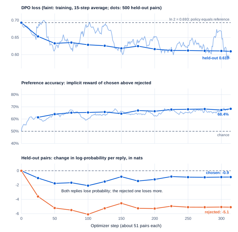
Five numbers per step say more than the loss: the loss; preference accuracy, the share of pairs whose chosen reply has the higher implicit reward; the reward margin, chosen minus rejected; and the chosen and rejected log-probabilities, separately. A loss of 0.6 can mean “chosen up, rejected down” or “both down, rejected faster”. Only the last two tell them apart.
Step 3: choosing the learning rate and β
Published settings
DPO runs use far smaller learning rates than supervised fine-tuning:
| Recipe | Learning rate | β | Batch (pairs) | Schedule and length |
|---|---|---|---|---|
| DPO paper (2023) | 1 × 10⁻⁶, RMSprop | 0.1 (0.5 for summarization) | 64 | warm-up over 150 steps |
| Zephyr-7B (2023) | 5 × 10⁻⁷ | 0.1 | 32 | linear, 10% warm-up, 1 to 3 epochs |
| Llama 3 (2024) | 10⁻⁵ | 0.1 | not given | plus an SFT loss on chosen replies, weight 0.2 |
| Tülu 3 8B (2024) | 5 × 10⁻⁷ | 5, length-normalized | 128 | linear, 10% warm-up, 1 epoch |
| SmolLM2 1.7B (2025) | 1 × 10⁻⁶ | 0.5 | 128 | 2 epochs, 1,024 tokens |
Tülu 3’s β of 5 isn’t comparable with the others, because its loss divides each log-ratio by the reply’s length. Hugging Face’s recipe for SmolLM2-135M and 360M uses the 1.7B model’s β and learning rate.
Learning-rate pilots
Four pilots ran on the first 2,000 pairs, β = 0.1: 40 steps of about 51 pairs, 3 warm-up steps, cosine decay to zero, each about 110 seconds. They were scored on 500 held-out pairs:
| Peak learning rate | Held-out loss | Accuracy | Chosen, change per token | Rejected, change per token |
|---|---|---|---|---|
| 1 × 10⁻⁶ | 0.677 | 61.0% | +0.0005 | -0.0010 |
| 3 × 10⁻⁶ | 0.662 | 61.2% | +0.0004 | -0.0032 |
| 1 × 10⁻⁵ | 0.652 | 62.2% | -0.0023 | -0.0107 |
| 3 × 10⁻⁵ | 0.707 | 61.0% | -0.0183 | -0.0318 |
Accuracy barely depends on the rate: about 61% after 40 steps at any of them. The loss does, and at 3 × 10⁻⁵ it rose past ln 2 = 0.693, worse than not training, because the pairs it got wrong it got confidently wrong. The last two columns show something the loss hides: at the two small rates the chosen replies gained probability, and from 1 × 10⁻⁵ up, both kinds lost it. The main run uses 1 × 10⁻⁵, ten times the DPO paper’s rate and equal to Llama 3’s.
At β = 0.1 the gradient norm ran from 10 to 56, so clipping at 1.0 rescaled every step. With AdamW that changes little, since Adam divides each update by a running estimate of the gradient’s size anyway.
β, swept
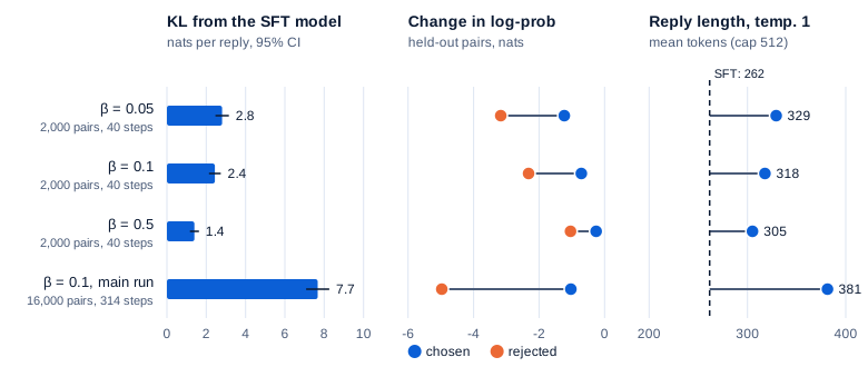
β prices the drift from the reference. Three short runs used the pilot setup at 1 × 10⁻⁵:
| β | Held-out accuracy (1,370 pairs) | Chosen, change per reply (nats) | Rejected, change per reply (nats) | KL from SFT per reply (nats) | Temperature-1 replies that end |
|---|---|---|---|---|---|
| 0.05 | 60.8% | -1.23 | -3.17 | 2.81 ± 0.34 | 79% |
| 0.1 | 60.7% | -0.71 | -2.32 | 2.44 ± 0.30 | 79% |
| 0.5 | 59.1% | -0.26 | -1.04 | 1.40 ± 0.23 | 83% |
The KL divergence is measured on the model’s own replies: sample a reply to each of 300 held-out prompts at temperature 1, sum log π minus log π_ref over its tokens, and average. Accuracy’s 95% interval on 1,370 pairs is about ±2.6 points, so the three runs tie on accuracy, but the KL halves from β = 0.05 to 0.5.
With Adam rescaling every update, β’s overall scale matters little. What matters is where each pair’s push switches off. The gradient on a pair is weighted by σ(-βΔ), with Δ the gap between the chosen and rejected log-ratios. At β = 0.5 a gap of 4 nats cuts that weight to 12%; at β = 0.05 it is still 45%, so a small β keeps pushing pairs the model already ranks correctly.
Swipe to pan the diagram, or tap it to zoom.
Smaller β gave longer replies: 329 tokens at β = 0.05, 305 at 0.5, from the SFT model’s 262. The main run kept β = 0.1, the DPO paper’s and Llama 3’s value, and with eight times the pairs it moved furthest on every measure.
Step 4: the main run
python dpo.py train --out runs/dpo88 --lr 1e-5 --beta 0.1 --limit 16000 --epochs 1 --budget 4096 \
--accum 13 --warmup 10 --val-every 25 --ckpt-every 50 --fused| Setting or result | Value |
|---|---|
| Model | 88,096,512 parameters, starting from Part 10’s SFT weights; reference: the same weights, frozen |
| Data | 16,000 UltraFeedback pairs, 1 epoch: 11.4M input tokens, 14.7M with padding |
| Batch and steps | 314 steps of 13 micro-batches of at most 4,096 padded tokens: about 51 pairs per step |
| Learning rate and β | 10 warm-up steps to 1 × 10⁻⁵, cosine to 0 at step 314; β = 0.1 |
| Optimizer | Part 5’s AdamW groups, betas (0.9, 0.95), epsilon 10⁻⁸, no weight decay, clipping at 1.0 (active on all 314 steps) |
| Precision and mode | BF16 autocast over FP32 weights, eager, fused AdamW, seed 1337 |
| Wall time | 14.1 minutes, including 14 held-out evaluations and 7 checkpoints; not resumed. The reference pass took 4.6 minutes more, once |
| Throughput | 20,359 padded tokens/s, 15,773 real tokens/s; MFU about 33% |
| Peak GPU memory | 4.66 GiB |
| GPU | SM clock median 2,070 MHz (90% between 1,920 and 2,160), memory 7,000 MHz (8,000 in 0.2% of samples), 49.7 W average, 81 °C median; nvidia-smi reported no power limit |
MFU (model FLOPs utilization) counts 6 FLOPs per parameter per real token against the 25.3 TFLOPS GPU Part 4 measured. The run is eager PyTorch, because Part 10 found torch.compile(dynamic=True) erratic on changing batch shapes. Hardware and software are the series’ usual: NVIDIA GeForce RTX 4060 Laptop GPU (8 GB), WSL2, driver 592.82, PyTorch 2.11.0 with CUDA 12.8.
Swipe to pan the diagram, or tap it to zoom.
Most of the gain came early: on the 500-pair subset, held-out accuracy was 64% at step 50 and 68.4% at the end. On all 1,370 held-out pairs the final model reaches 67.6%.
Both replies lose probability
At the end, the average held-out chosen reply had lost 1.03 nats against the reference, and the rejected reply 4.97. The chosen reply’s probability fell in 58% of pairs, the rejected reply’s in 79%. DPO widened the gap mostly by pushing rejected replies down, and pushed chosen replies down too.
This is the widely reported part of DPO. The DPO authors, in From r to Q*, call it “a well observed phenomena in which the likelihood of the chosen responses actually decrease over time”: averaged over replies the reference would write, the implicit reward equals minus β times a KL divergence, so implicit rewards “must decrease in expectation”. Razin et al. named it likelihood displacement and showed it can do harm: “training a model to prefer No over Never can sharply increase the probability of Yes”. Llama 3’s extra loss on chosen replies is there to prevent “the decrease of log probability of chosen responses”.
The probability that left both replies had to go somewhere, and the next two sections show part of it going to stopping later.
Longer replies
On 500 held-out prompts, sampled, the SFT model’s replies that ended had a median of 242 tokens and the DPO model’s 352; only 65% ended within 512 tokens, against 85%. The training data predicts the direction: chosen replies are longer in 56.7% of pairs. DPO overshot it. On the same 500 prompts the chosen replies average 268 tokens, the rejected ones 226 and the SFT model’s samples 267, while the DPO model’s samples average 385 even when cut off at 512.
Park et al. found the same with Pythia 2.8B on dialogue and summarization data: where the data shows “a small bias in preference towards longer responses, the un-regularized DPO model produces answers twice as long on average”, “significantly longer than both the preferred and rejected answers”.
Where the stopping went
The <|end|> token closes every chosen and every rejected reply, so each pair pushes it up in one reply and down in the other. The net effect, on the 1,370 held-out pairs:
| Log-probability (nats) | SFT model | DPO model | Change |
|---|---|---|---|
<|end|> closing a chosen reply | -2.87 | -3.24 | -0.37 |
<|end|> closing a rejected reply | -2.80 | -3.66 | -0.86 |
| Other tokens of chosen replies, per token | -2.478 | -2.481 | -0.003 |
| Other tokens of rejected replies, per token | -2.416 | -2.434 | -0.018 |
In chosen replies, the end token fell over 100 times as far as an ordinary token. One reading: rejected replies are shorter, so “stop here” is usually the losing move. Llama 3 masked “special formatting tokens including header and termination tokens” out of its DPO loss, because letting them count “may lead to undesired model behaviors such as tail repetition or abruptly generating termination tokens”. Masking <|end|> here is a one-line change to collate_pairs, not tested in this part.
Step 5: before and after
Measured without a judge
| Measure | SFT model (Part 10) | DPO model |
|---|---|---|
| Held-out pairs: implicit-reward accuracy (1,370 pairs) | none: both rewards are 0 | 67.6% |
| Held-out pairs: chosen more likely than rejected, by total log-probability | 41.2% | 41.8% |
| Same, per token | 47.7% | 49.7% |
| KL from the SFT model per reply, temperature 1 (300 prompts) | 0 | 7.67 ± 0.59 nats (0.020 per token) |
| Held-out prompts, sampled: replies that end within 512 tokens (500 prompts) | 85.0% | 65.2% |
| Same: median length of replies that ended | 242 tokens | 352 tokens |
| Same: repeated 4-token sequences | 19% | 23% |
| Held-out prompts, greedy: replies that end | 48.2% | 25.8% |
| Same: repeated 4-token sequences | 65% | 76% |
| Part 10’s 100 prompts, greedy: replies that end within 256 tokens | 33% | 12% |
| Same, sampled | 39% | 20% |
| HellaSwag acc_norm | 28.0 ± 0.9 | 27.9 ± 0.9 |
| ARC-Easy acc | 44.1 ± 2.0 | 44.6 ± 2.0 |
| PIQA acc | 58.6 ± 2.3 | 58.7 ± 2.3 |
Sampling uses temperature 0.8 and top-k 50, as in Part 10, through a new batched sampler with a key-value cache, sampling.py; its tie-breaking explains the SFT model’s 33% here against Part 10’s 36%. The benchmarks are Part 9’s, zero-shot, and the SFT scores are Part 10’s.
The benchmarks didn’t move; every change is inside its interval. The alignment tax, the drop in existing abilities caused by post-training, was zero. Everything else moved the wrong way for a user: replies got longer, ended less often and repeated themselves more.
A small judge
Skywork-Reward-V2-Qwen3-0.6B is an Apache 2.0 Bradley-Terry reward model built on Qwen3-0.6B, trained, per its card, on “26 million preference pairs”; in BF16 it takes 1.2 GB. On the 1,370 held-out pairs it agrees with UltraFeedback’s GPT-4-based labels 78.0% of the time, scoring chosen replies 2.59 on average and rejected ones -0.01.
Our two models score -10.0 (SFT) and -10.8 (DPO) on 500 held-out prompts: Step 1’s quality gap, in one number. Head to head on each prompt, the judge preferred the DPO model’s sampled reply 37.1% ± 4.2% of the time, and its greedy reply 39.1% ± 4.2%. One 0.6B judge is a weak proxy, and it marks down replies cut off at the length limit, which the DPO model writes more often.
What the model writes
The same prompts as Part 10, greedy and sampled with temperature 0.8, top-k 50 and seed 0, limited to 200 new tokens. Replies are quoted verbatim and trimmed:
| Prompt | SFT model, greedy | DPO model, greedy |
|---|---|---|
| What is the capital of France? | “The capital of France is Paris. It is a city known for its rich history, culture, and culture.” (no end) | “The capital of France is Paris, a city located in the heart of the Mediterranean Sea.” (no end) |
| Give me three tips for sleeping better. | “Here are some tips to help you sleep better: 1. **Sleeping**: Make sure your body is in good shape, and your body is in good shape.” (no end) | “Here are some tips to help you get started: 1. Sleep: Aim for 3-6 hours of sleep each night.” (no end) |
| Rewrite this sentence to sound more formal: hey, can u send me the report by tmrw? | “The sentence “hey” is a contraction of “hey” in the context of the sentence.” (ends, 54 tokens) | “The sentence “hey, can u send me the report by tmrw?” is a classic example of a formal formal formal formal formal…” (no end) |
| What was the weather like in Pune yesterday? | “In Pune yesterday, the weather was quite mild, with a slight chill.” (no end) | “In Pune, the weather was quite mild, with temperatures ranging from 30°C to 40°C.” (no end) |
| What is 17 + 25? | “To find 17 + 25, we can use the concept of a sequence of numbers.” (no end) | “The sum of the given numbers is 17 + 25 = 17.” (no end) |
Across the nine prompts, greedy and sampled, the SFT model ended 7 of 18 replies within 200 tokens and the DPO model 1. Neither is more correct: Paris has moved to the Mediterranean, and 17 + 25 is now 17.
On-policy pairs: same loss, opposite result
Off-policy pairs teach the model on text it wouldn’t write. The usual fix, used by both Llama 3 and Tülu 3, is on-policy pairs: sample replies from the model itself and let a judge rank them, so the rejected replies carry the model’s real failures, the loops and the missing ends.
The SFT model wrote four temperature-1 replies of up to 384 tokens to each prompt, 64 replies per batch. The first batch took 16.9 seconds, so 2,000 prompts would have taken 35 minutes; to fit the GPU budget the run kept the first 704, 2,816 replies in 14 minutes. The reward model scored them in 100 seconds, and its best and worst reply per prompt became the pair. These pairs lean the other way from UltraFeedback’s: the chosen reply is longer in only 23% of them, 207 tokens against 295 on average, and ended in 88% of pairs against 62%.
A control run trained on the UltraFeedback pairs of the same 704 prompts. Both used β = 0.1, a peak learning rate of 1 × 10⁻⁵ and a 3-step warm-up, for 3 epochs, 42 steps. Both memorized their pairs by the end, but on first sight the on-policy run ranked 65% of pairs correctly and the off-policy run 56%: the on-policy signal is easier to learn.
| Measure | SFT model | Off-policy, 704 prompts | On-policy, 704 prompts | Main run, 16,000 pairs |
|---|---|---|---|---|
| UltraFeedback held-out pairs: implicit-reward accuracy | none | 60.0% | 42.3% | 67.6% |
| KL from the SFT model per reply (nats) | 0 | 4.17 ± 0.39 | 4.69 ± 0.35 | 7.67 ± 0.59 |
| Temperature-1 replies: end within 512 tokens | 91% | 76% | 99.7% | 67% |
| Temperature-1 replies: mean length | 262 | 345 | 81 | 381 |
| Sampled replies: median length of those that ended | 242 | not run | 53 | 352 |
| Greedy replies that end, held-out prompts | 48.2% | not run | 80.4% | 25.8% |
| Greedy replies: repeated 4-token sequences | 65% | not run | 34% | 76% |
| Greedy replies that end, Part 10’s prompts | 33% | not run | 73% | 12% |
| HellaSwag / ARC-Easy / PIQA | 28.0 / 44.1 / 58.6 | not run | 27.9 / 43.3 / 58.5 | 27.9 / 44.6 / 58.7 |
| Reward-model judge: beats the SFT reply (sampled) | reference | not run | 77.3% ± 3.6% | 37.1% ± 4.2% |
With the same loss and settings, the replies went the opposite way: 81 tokens on average against 345, nearly every reply ending, greedy repeats halved. Asked for the capital of France, the on-policy model writes “The capital of France is Paris.” and stops after 8 tokens. Asked to rewrite the casual sentence formally, it answers “I’m sorry for the confusion, but as a writer, I don’t have the ability to read the text.” The data, not DPO, set the direction.
The judge’s 77% needs a warning: the same reward model built the pairs and judged the result, so it favors this arm by construction. The checks that don’t depend on it agree on the main point. End rate, repetition and length moved toward the stopping that Part 10’s model only half learned, the benchmarks stayed inside their intervals, and the KL per reply stayed below the main run’s (per token it is higher, 0.057 nats, because the replies are short). They also show the cost. Median replies of 53 tokens are short for many prompts, and on UltraFeedback’s held-out pairs the on-policy model now moves toward the GPT-4-rejected reply in 58% of pairs, because those labels favor length and this judge favored stopping. One run per arm, 704 prompts and a 0.6B judge are enough to show the direction, not to settle details such as how many epochs to run.
In the real world
- Llama 3 ran DPO in each of six rounds, on “the most recent batches of preference data collected using the best performing models from the previous alignment rounds”, so the data “conforms better to the distribution of the policy model”. Each round also used rejection sampling: “we sample K (typically between 10 and 30) outputs from the latest chat model policy” and keep the reward model’s favorite (Llama Team, 2024).
- Tülu 3 extended UltraFeedback’s recipe to a pool of 22 models graded by GPT-4o and added on-policy pairs, where one reply comes from its own SFT model: 96,911 off-policy and 19,444 on-policy pairs in its base mix. It found that “only length-normalized DPO outperformed our base checkpoint overall” (Lambert et al., 2024).
- Zephyr-7B ran DPO for three epochs on UltraFeedback and “observed that after one epoch of DPO training, the model would strongly overfit”, yet “this did not harm downstream performance on MT-Bench and AlpacaEval” (Tunstall et al., 2023).
What DPO can’t do is visible at 88M. It reweights replies the model can already write, in whatever direction the pairs point. On UltraFeedback that direction was length, the easiest signal in the data; on its own replies ranked by a reward model, it was stopping. Neither run added knowledge.
Part 12’s reinforcement learning with verifiable rewards (RLVR) changes the source of the signal. The model answers questions whose answers a program can check, and GRPO, derived in Math Part 16, pushes up the answers that beat their group’s average. The data is on-policy by construction, and a checker, with no taste to exploit, sets the reward.
Common misconceptions
- “DPO decides what the model learns.” The pairs do. Same loss and settings: off-policy pairs grew replies to 345 tokens, on-policy pairs shrank them to 81.
- “DPO raises the probability of the chosen reply.” It raises the gap. Here the chosen reply’s log-probability fell in 58% of held-out pairs, by 1.03 nats on average; the rejected reply fell further.
- “Preference accuracy measures how good the model is.” It measures whether the policy moved away from the reference in the labeled direction. The main DPO model reached 67.6%, while a reward model preferred its replies to the SFT model’s only 37% of the time; the on-policy model scored 42% on the same pairs and won 77%.
- “DPO needs a second model in memory.” It needs the reference’s log-probabilities. For a fixed set of pairs they can be computed once, 4.6 minutes here, and the reference never touches the training loop.
Key takeaways
- A preference pair is a prompt, a chosen reply and a rejected reply. UltraFeedback’s 61,135 pairs come from 17 models graded by GPT-4; after filtering, 41,755 fit this model.
- The DPO loss needs four log-probabilities per pair. The reference’s two never change, so compute them once and keep only the policy in memory.
- Log the chosen and rejected log-probabilities separately. Here both fell, by 1.0 and 5.0 nats per reply, while held-out accuracy rose to 67.6%.
- DPO follows what the pairs reward. UltraFeedback’s length bias made replies about 45% longer and far fewer ending; the model’s own replies, ranked by a reward model, pushed 97% of replies to end, and that same reward model judged them better 77% of the time.
- Benchmarks didn’t move. The alignment tax of this stage was zero, and so was its gain in knowledge.
What’s next
Part 12 replaces preferences with a checker. The model will answer arithmetic and format questions, a few lines of Python will grade every answer, and GRPO will push up the answers that beat their group’s average, all on the model’s own samples, with reward curves you can watch climb or stall.
Further reading
- Direct Preference Optimization: Your Language Model is Secretly a Reward Model (Rafailov et al., 2023): the loss, its derivation and the default settings.
- From r to Q*: Your Language Model is Secretly a Q-Function (Rafailov et al., 2024): Section 5.4, why likelihoods should fall during DPO.
- Unintentional Unalignment: Likelihood Displacement in Direct Preference Optimization (Razin et al., 2024): when falling likelihoods move probability somewhere harmful.
- Smaug: Fixing Failure Modes of Preference Optimisation with DPO-Positive (Pal et al., 2024): how pairs with small differences push chosen replies down.
- Disentangling Length from Quality in Direct Preference Optimization (Park et al., 2024): DPO’s length exploitation and a length-regularized fix.
- UltraFeedback: Boosting Language Models with Scaled AI Feedback (Cui et al., 2023) and the binarized dataset card: where the pairs come from.
- Zephyr: Direct Distillation of LM Alignment (Tunstall et al., 2023): DPO on UltraFeedback at 7B, with its settings.
- Tülu 3: Pushing Frontiers in Open Language Model Post-Training (Lambert et al., 2024): on-policy preference data and length-normalized DPO.
- The Llama 3 Herd of Models (Llama Team, Meta, 2024): Section 4, rounds of rejection sampling and DPO.
- SmolLM2: When Smol Goes Big (Ben Allal et al., 2025) and its DPO recipe for the small models: DPO settings for models near this size.
- Skywork-Reward-V2-Qwen3-0.6B model card: the small open reward model used as a judge here.
- RLHF Book (Nathan Lambert): a free book on reward models, DPO and RL with verifiable rewards.