
LLM Inference & Optimization · Part 9 of 14
Speculative Decoding: Guess Several Tokens, Check Them in One Pass
Why checking several guessed tokens costs about as much as writing one, how speculative sampling keeps the output exact, and Medusa, EAGLE and MTP.
On this page
TL;DR
During decode, a GPU reads every weight of the model to produce a single token while its arithmetic units sit almost idle. Speculative decoding uses that idle arithmetic. A cheap drafter guesses the next few tokens, and the big model checks all of them in one forward pass, which costs about as much as generating one token. The big model keeps the guesses up to the first one it disagrees with and writes its own token there, so each expensive pass yields several tokens. A rejection-sampling rule called speculative sampling makes the output distribution exactly the big model’s, so quality is unchanged. By the end you’ll be able to estimate the speedup from the acceptance rate, know where drafts come from (small models, Medusa heads, EAGLE, DeepSeek’s multi-token prediction, text lookup), and see why the gain shrinks as batches grow.
Why it matters
Part 1 set a speed limit. Llama 3.1 8B on an NVIDIA H100 has to read 16 GB of weights for every token it writes, so a single user can’t get more than about 208 tokens per second, however fast the arithmetic is.
Then the SGLang team ran that same model on one H100 and measured 373 tokens per second for a single user. Their baseline without the trick was 158. The weights and the hardware were the same, and the output follows the same probability distribution as before.
The trick is speculative decoding, which gets more than one token out of each trip to memory. vLLM, SGLang and TensorRT-LLM all ship it, DeepSeek trained its V3 model with a module that can drive it, and OpenAI’s API lets you supply the guesses yourself.
The intuition
Picture a senior author dictating a book one word at a time. Each word takes a few seconds.
Now add an apprentice who knows the author’s style and can write the next four words in a moment. The author reads them in one glance, which takes about as long as producing one word, nods at the first two, frowns at the third and says the word they would have used. That’s three words for the price of one. A good apprentice gets mostly nods. A bad one gets corrected on the first word every time, and you’re back to one word per glance plus the apprentice’s wasted effort.
The analogy breaks in two places. The glance is cheap only because of how GPUs work: reading the weights dominates the cost, and checking four words reads them once, just like writing one. And a real model has probabilities over thousands of tokens instead of one right word, so “nodding” has to be a precise probabilistic rule, or the book would drift toward the apprentice’s style.
Step 1: why checking is almost free
Recall Part 1’s numbers for Llama 3.1 8B (8.03 billion parameters, 16-bit weights) on an H100 (989 trillion floating-point operations, or FLOPs, per second; 3.35 TB/s of memory bandwidth):
weights read per decode step  = 16.06 GB ÷ 3.35 TB/s       ≈ 4.79 ms
math for 1 token              = 2 × 8.03 billion = 16 GFLOP ≈ 0.016 ms
Now feed the model 5 positions in one pass instead of 1: the last real token plus 4 guessed tokens. The weights are still read once, and the math grows five times:
math for 5 positions = 2 × 8.03 billion × 5 = 80 GFLOP ≈ 0.08 ms
step time            ≈ max(4.79 ms memory, 0.08 ms math) ≈ 4.79 ms
Even if the math didn’t overlap with the memory reads at all, checking 4 guesses would add 0.065 ms to a 4.79 ms step, about 1.4%. In roofline terms the pass does 5 FLOPs per byte of weights instead of 1, far below the 295 FLOPs per byte the H100 (Part 3) needs before arithmetic becomes the limit. The KV cache (the stored keys and values of earlier tokens, Part 2) is read once too, since the 5 positions belong to one sequence: about 0.16 ms at 4,096 tokens of context.
The 5-position pass works like a tiny prefill, attention kernels and all (Part 7). Through the causal mask, each position sees only the tokens before it, so one pass predicts what follows the real token, what follows guess 1, and so on: exactly what’s needed to grade every guess.
Leviathan, Kalman and Matias at Google, who published the method in 2022, note that decoding K tokens “takes K serial runs of the model.” Speculative decoding turns most of those serial runs into one parallel run.
Step 2: draft, verify, accept
Each step of the loop has three parts:
- Draft: a cheap draft model proposes
ktokens, one after another. Each of its steps is fast. - Verify: the large target model, whose output you actually want, runs once over the last accepted token plus the
kdrafts and producesk + 1predictions. - Accept: walk through the guesses in order and keep each one the target agrees with. At the first disagreement, discard that guess and everything after it, and emit the target’s own token instead.
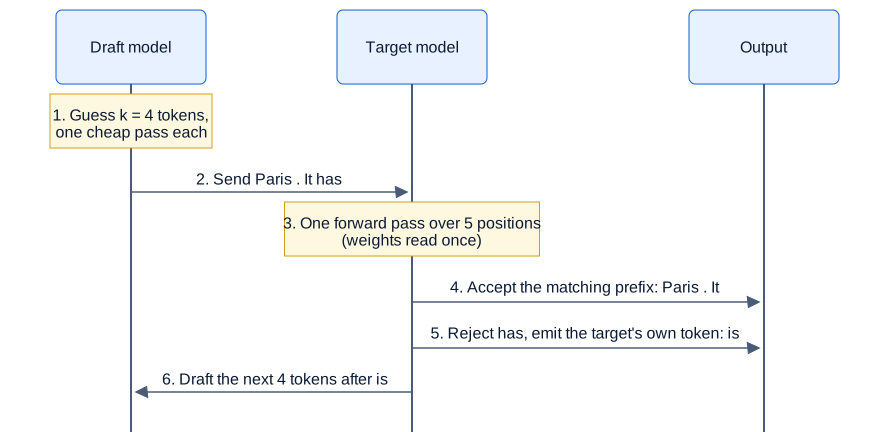
Swipe to pan the diagram, or tap it to zoom.
Here one target pass produced four tokens, where plain decoding would have produced one.
A worked example with greedy decoding
Start with greedy decoding, where the model always takes its single most likely token (Fundamentals Part 1 covers it). The prompt is “The capital of France is”, and the draft proposes 4 tokens. The target’s pass gives its top choice at each of the 5 positions:
| Position | Draft’s guess | Target’s top choice at this position | Result |
|---|---|---|---|
| 1 | ” Paris” | ” Paris” | Accept |
| 2 | ”.” | ”.” | Accept |
| 3 | ” It” | ” It” | Accept |
| 4 | ” has” | ” is” | Reject, emit ” is” |
| 5 | (nothing left to check) | ” a” | Ignored: it assumed ” has” |
The step outputs ” Paris. It is”: 3 accepted guesses plus 1 correction. The prediction at position 5 is useless, because the target made it assuming ” has” came before it. Had all four guesses matched, that fifth prediction would have been valid too, a free bonus token, so a step yields between 1 and k + 1 tokens.
The rule fits in a few lines:
def verify_greedy(draft, target_picks):
    # target_picks[i] is the target's top token at position i, given the prompt
    # plus draft[:i]. There are k + 1 of them for k drafted tokens.
    out = []
    for guess, pick in zip(draft, target_picks):
        if guess != pick:
            out.append(pick)          # first mismatch: keep the target's token, stop
            return out
        out.append(guess)             # match: accept the draft token
    out.append(target_picks[-1])      # every guess matched: one bonus token
    return out

verify_greedy([" Paris", ".", " It", " has"], [" Paris", ".", " It", " is", " a"])
# [' Paris', '.', ' It', ' is']
Every output token is one the target would have chosen anyway. A terrible draft still yields one correct token per step, so the worst case costs drafting time and leaves quality alone.
What happens to the rejected tokens
The verify pass wrote keys and values for all 5 positions into the KV cache, and the entries for ” has” and the position after it are now wrong. The engine rolls the sequence length back and the next step overwrites those slots; with a paged cache (Part 5), that means trimming the last block. The draft model keeps a KV cache of its own, which takes memory: on an RTX 3090 with 24 GB, the EAGLE paper’s 7B setup fit a batch of 8 without speculation and 7 with it.
Step 3: speculative sampling keeps the output exact
Greedy decoding is the easy case. Chat models usually sample: they draw the next token at random from the model’s probabilities, often reshaped by temperature or top-p. With no single right token, “accept if it matches” stops making sense.
Leviathan et al. and Chen et al. at DeepMind (2023) solved this independently; Chen et al. called it speculative sampling. Write p(x) for the target’s probability of token x and q(x) for the draft’s (Chen et al. swap the letters; this follows Leviathan). For each drafted token x, in order:
- Accept
xwith probabilitymin(1, p(x) / q(x)). - If it’s rejected, sample a replacement from
norm(max(0, p − q)): subtract the draft’s probabilities from the target’s, set negatives to zero, and rescale so they sum to 1. Then stop and discard the later drafts. - If every draft was accepted, sample a bonus token from the target’s last distribution.
If the draft was less confident in a token than the target is (q ≤ p), the token is always kept. If the draft was overconfident, it’s kept only part of the time, and a rejection draws from the tokens the draft under-proposed.
A three-token example
Take the prompt “The sky is” and a vocabulary of three tokens. The target and draft disagree:
| Token | Target p | Draft q | Accept probability min(1, p/q) | Residual max(0, p − q), normalized |
|---|---|---|---|---|
| ” blue” | 0.5 | 0.3 | 1 | 0.2 → 2/3 |
| ” grey” | 0.2 | 0.5 | 0.4 | 0 → 0 |
| ” clear” | 0.3 | 0.2 | 1 | 0.1 → 1/3 |
The draft likes ” grey” (0.5) far more than the target does (0.2), so a proposed ” grey” survives only 40% of the time. After a rejection, the replacement comes from ” blue” and ” clear”, the tokens the draft proposed too rarely, in the ratio 2 to 1. Simulating a million draws:
import numpy as np
rng = np.random.default_rng(0)
p = np.array([0.5, 0.2, 0.3])   # target: blue, grey, clear
q = np.array([0.3, 0.5, 0.2])   # draft

def speculative_sample():
    x = rng.choice(3, p=q)                    # draft proposes
    if rng.random() < min(1, p[x] / q[x]):    # accept with prob min(1, p/q)
        return x, True
    r = np.maximum(p - q, 0); r /= r.sum()    # residual distribution
    return rng.choice(3, p=r), False

draws = [speculative_sample() for _ in range(1_000_000)]
print(np.bincount([x for x, _ in draws]) / 1e6)   # [0.500 0.200 0.300]
print(np.mean([ok for _, ok in draws]))           # 0.700: acceptance rate
The output frequencies match the target’s 0.5, 0.2 and 0.3, although every candidate came from the draft. The acceptance rate, 0.70, is the sum of min(p, q) over the vocabulary: 0.3 + 0.2 + 0.2.
Why it’s exact
A step can output token x in two ways: the draft proposed x and it was kept, or something was rejected and x was drawn as the replacement.
P(x) = q(x) × min(1, p(x)/q(x))  +  (1 − α) × max(0, p(x) − q(x)) / (1 − α)
     = min(p(x), q(x))           +  max(0, p(x) − q(x))
     = p(x)
Here α = Σ min(p, q) is the chance of accepting. The chance of rejecting, 1 − α, also equals the total mass of max(0, p − q), which is why the two cancel. The last line holds because min(p, q) + max(0, p − q) equals p for any two numbers. The argument repeats position by position, so the whole sequence follows the target’s distribution. Greedy decoding is the special case where p puts all its probability on one token: min(1, p/q) is then 1 for that token and 0 for the rest, which is the matching rule from Step 2.
Temperature, top-k and top-p all fit, as long as p and q are the distributions after those settings are applied; Leviathan et al. note that all of them “can easily be cast into standard sampling from an adjusted probability distribution.” vLLM’s docs describe the result as “theoretically lossless up to the precision limits of hardware numerics,” meaning the same distribution give or take floating-point rounding.
Step 4: how much faster, and when it hurts
Tokens per verify step
Let α be the average acceptance rate, the chance that the target keeps a drafted token. Leviathan et al. assume each guess is accepted independently with probability α. A step with k drafts then produces, on average:
E(tokens per step) = (1 − α^(k+1)) / (1 − α)With α = 0.8 and k = 4: (1 − 0.8^5) / 0.2 = (1 − 0.328) / 0.2 = 3.36 tokens per target pass. The formula is a geometric series. You always get the first token (a correction or the first accept), the second with probability α, the third with α², and so on up to k + 1.
| Acceptance rate α | k = 2 | k = 3 | k = 4 | k = 5 | k = 6 | k = 7 | k = 8 | Limit (k → ∞) |
|---|---|---|---|---|---|---|---|---|
| 0.6 | 1.96 | 2.18 | 2.31 | 2.38 | 2.43 | 2.46 | 2.47 | 2.5 |
| 0.8 | 2.44 | 2.95 | 3.36 | 3.69 | 3.95 | 4.16 | 4.33 | 5 |
| 0.9 | 2.71 | 3.44 | 4.10 | 4.69 | 5.22 | 5.70 | 6.13 | 10 |
The acceptance rate matters more than the draft length. At α = 0.6, no draft length gets past 2.5 tokens per step, because 1 / (1 − α) caps it. Longer drafts also pay off less and less: going from 4 to 8 drafts at α = 0.8 adds under one token per step, since the later guesses are rarely reached.
Paying for the draft
Let c be the time of one draft step as a fraction of one target step. A full cycle costs k draft steps plus one target pass, (k × c + 1) target-step units, so the speedup over plain decoding is:
speedup = (1 − α^(k+1)) / ((1 − α) × (k × c + 1))This is Leviathan et al.’s walltime formula. For a concrete draft, take Llama 3.2 1B (1.24 billion parameters, same tokenizer) drafting for Llama 3.1 8B. If its step time scaled with its weight bytes, as memory-bound decode does, c ≈ 1.24 / 8.03 ≈ 0.15. The speedup for a few values of c:
| Acceptance rate α | Draft cost c | k = 1 | k = 2 | k = 4 | k = 6 | k = 8 | Best k |
|---|---|---|---|---|---|---|---|
| 0.6 | 0.05 | 1.52 | 1.78 | 1.92 | 1.87 | 1.77 | 4 |
| 0.6 | 0.15 | 1.39 | 1.50 | 1.43 | 1.26 | 1.11 | 2 |
| 0.8 | 0.05 | 1.71 | 2.22 | 2.80 | 3.04 | 3.09 | 8 |
| 0.8 | 0.15 | 1.56 | 1.87 | 2.08 | 2.05 | 1.94 | 4 or 5 |
| 0.9 | 0.15 | 1.65 | 2.07 | 2.53 | 2.71 | 2.75 | 8 |
At α = 0.8, k = 4 and c = 0.15, the speedup is 2.08, which would lift Part 1’s ceiling of 208 tokens per second to about 430. A cheaper drafter pushes the best k up, and a weak or slow one pushes it down to 1 or 2. Small models also pay fixed costs per step, such as kernel launches, so their real c is usually above the byte ratio. That’s why later drafters live inside the target model.
Wasted work, and why batching changes the answer
Every rejected guess was still computed. At α = 0.8 and k = 4, the target processes 5 positions to keep 3.36 tokens, about 1.5 times the arithmetic per output token; at α = 0.6 it’s 2.2 times. In single-user decode that arithmetic was idle anyway, so the waste is free. At larger batches it isn’t.
Part 4 showed how servers batch many users into each step to use the idle arithmetic, so batching and speculation compete for the same spare capacity. With B users and k drafts each, the verify pass processes B × (k + 1) positions, and Part 1’s ridge point says the H100 becomes compute-bound at about 295 positions per pass. Here’s our own roofline estimate for Llama 3.1 8B on an H100, counting weight reads only, with α = 0.8, k = 4 and a light drafter at c = 0.05:
| Users in the batch | Positions per verify pass | Tokens/s without speculation | Tokens/s with speculation | Speedup |
|---|---|---|---|---|
| 1 | 5 | 209 | 584 | 2.80× |
| 32 | 160 | 6,675 | 18,699 | 2.80× |
| 64 | 320 | 13,350 | 34,953 | 2.62× |
| 128 | 640 | 26,700 | 37,905 | 1.42× |
| 256 | 1,280 | 53,400 | 39,577 | 0.74× |
| 512 | 2,560 | 61,582 | 39,810 | 0.65× |
Up to about 59 users, the 5 positions per user stay under the ridge and speculation is a near-free 2.8×. Beyond that, each verify pass takes longer and the wasted arithmetic costs real time; by 256 users, speculation is slower than plain batching. Real decode also reads the KV cache, which keeps steps memory-bound longer and moves the crossover to bigger batches, but the measurements below have the same shape.
In the real world
Separate draft models
The original papers used off-the-shelf models from the same family. Leviathan et al. sped up T5-XXL (11 billion parameters) with T5-small (77 million) as the drafter. On English-to-German translation with greedy decoding, α was 0.75 with k = 7, and the speedup 3.4× at batch size 1 on a single TPU v4; sampling at temperature 1 gave α = 0.62 and 2.6×. Their c “was always less than 0.05.” Chen et al. built a 4 billion-parameter drafter for Chinchilla 70B: 1.8 ms per token against the target’s 14.1 ms on 16 TPU v4s (c ≈ 0.13). With k = 4 at batch size 1, they got 1.92× to 2.01× on XSum summarization and 2.46× on HumanEval code generation. The draft should use the target’s tokenizer; TensorRT-LLM’s docs warn that otherwise “the acceptance rate is extremely low and performance is regressed.”
Heads and layers on the target: Medusa and EAGLE
Medusa (Cai et al., 2024) adds small output heads to the target’s final layer. Head 1 guesses the token after next, head 2 the one after that, and their guesses form a tree of candidate continuations that tree attention, a custom attention mask, verifies in one pass. Training only the heads on a frozen model (Medusa-1) gave 2.18× on Vicuna-7B and 2.33× on Vicuna-13B at batch size 1. Training heads and model together (Medusa-2) gave 2.83× on both, peaking at 3.62× on MT-Bench’s extraction category. Medusa’s optional “typical acceptance” rule gives up exactness when sampling.
EAGLE (Li et al., 2024) drafts with about one decoder layer that reads the target’s hidden state just below the output head, plus the token sequence shifted one step ahead. It reported 2.7× to 3.5× lower latency for LLaMA2-Chat 70B with the output distribution unchanged. EAGLE-2 grows the draft tree where the drafter is confident and reported 3.05× to 4.26×, 20 to 40% faster than EAGLE-1. EAGLE-3 (2025) predicts tokens directly from features fused across several of the target’s layers. It reports up to 6.5×, on Vicuna 13B for HumanEval at temperature 0, and 4.40× for Llama 3.1 8B on MT-Bench, at 6.13 tokens per verify step on average. Both families need a drafter trained for each target; for a 70B model, EAGLE’s training takes 1 to 2 days on four A100 40 GB GPUs.
Multi-token prediction
Gloeckle et al. at Meta (2024) trained models from the start with several output heads, each predicting a token further ahead. Used as their own drafter in greedy self-speculative decoding, their 7B model with 4-token prediction ran 3.0× faster on code, accepting 2.5 of 3 suggested tokens on average, and 2.7× faster on text. DeepSeek-V3 trained one extra MTP module that predicts the token after next. Used for speculative decoding, “the acceptance rate of the second token prediction ranges between 85% and 90%,” delivering “1.8 times TPS” (tokens per second). The formula agrees: with k = 1, 1 + α gives 1.85 to 1.9 tokens per step. Part 14 returns to it as part of DeepSeek’s inference stack.
Drafts without a model
When the output repeats the input, the draft can be copied from the prompt. Prompt lookup decoding, by Apoorv Saxena, finds the last few generated tokens somewhere in the prompt and proposes whatever followed them there. It targets “input grounded generation” such as summarization, document question answering, code editing and retrieval-augmented answers. On Mistral-7B-Instruct with greedy decoding on one A100, summarization and context question answering ran about 2.4× faster on average. Like prefix caching, it’s a bet on repetition.
OpenAI’s Predicted Outputs let you hand in a guess yourself, such as the current file when you ask for one property to be renamed. OpenAI doesn’t document the mechanism, but the usage report counts prediction tokens as accepted or rejected, and “any rejected tokens are still billed like other completion tokens.” It works with the GPT-4o and GPT-4.1 series.
Lookahead decoding (Fu et al., 2024) makes its own candidate n-grams (short runs of tokens) by iterating guesses for several future positions in parallel inside the target model, then verifies them like any draft. Without a draft model or training, it measured up to 1.8× on MT-Bench and up to 4× on code completion across multiple A100 GPUs.
Turning it on
- vLLM takes a
speculative_configwhosemethodcan be"draft_model","eagle","eagle3","mtp","ngram"or"suffix", withnum_speculative_tokensask. Its docs pitch it for reducing “inter-token latency under medium-to-low QPS (queries per second), memory-bound workloads.” - SGLang uses
--speculative-algorithmwithEAGLE,EAGLE3,STANDALONE(a separate draft model) orNGRAM, and recommends EAGLE-3 for “Best speed/quality.” Models with built-in MTP heads run through its EAGLE path. - TensorRT-LLM has config classes for draft-target, EAGLE-3, MTP, n-gram and others. Its docs open with: “Speculative decoding is a technique for accelerating LLM inference at low batch sizes.”
vllm serve meta-llama/Llama-3.1-8B-Instruct \
  --speculative-config '{"method": "ngram", "num_speculative_tokens": 4,
                         "prompt_lookup_min": 2, "prompt_lookup_max": 5}'
It stacks with other optimizations. EAGLE combined with gpt-fast’s 4-bit quantization ran LLaMA2-Chat 7B at 160.4 tokens per second on a single RTX 3090, against 24.5 for the plain Hugging Face implementation in 16-bit.
What happens at larger batches
The SGLang team ran EAGLE-3 with Llama 3.1 8B on one H100 at growing batch sizes, as reported in the EAGLE-3 paper:
| Batch size | 2 | 4 | 8 | 16 | 32 | 64 |
|---|---|---|---|---|---|---|
| EAGLE throughput vs no speculation | 1.40× | 1.38× | 1.23× | 1.02× | 0.94× | 0.99× |
| EAGLE-3 throughput vs no speculation | 1.81× | 1.82× | 1.62× | 1.48× | 1.32× | 1.38× |
The gain shrinks as the batch grows, and the older EAGLE dips slightly below break-even from batch 24 on. The vLLM team saw the same in 2024. On Llama 3 70B with four H100s, a draft model gave up to 1.5× at 1 request per second on ShareGPT conversations, and prompt lookup up to 2.8× on CNN/DailyMail summaries. At high request rates the same setups were 1.4× and 1.8× slower, because “the extra compute required to propose and verify tokens can sometimes slow down the system when it is already compute-bound.” vLLM now offers dynamic speculative decoding for “workload with fluctuating QPS.”
Common misconceptions
- “Speculative decoding trades quality for speed.” With speculative sampling, the output follows the target’s distribution exactly, up to floating-point rounding, and a bad drafter only costs speed. Lossy variants, such as Medusa’s typical acceptance or vLLM’s FLy verification, are opt-in and labeled.
- “It speeds up time to first token.” It speeds up decode only. The prompt still goes through one prefill, so the first token arrives no sooner. How to Reduce Time to First Token covers what does help.
- “More draft tokens is always better.” Returns fall off as
α^k, and every extra guess costs draft time and verify arithmetic. With a 0.15-cost drafter atα = 0.6, the best draft length is 2. - “It always increases throughput.” It spends idle arithmetic, which is free at small batches and already in use at large ones, where speculation can cut throughput, as vLLM measured. Treat it as a latency tool.
- “The draft model must be small and separate.” Medusa heads, EAGLE layers, MTP modules, a prompt lookup or your own predicted text all work as drafts.
Key takeaways
- Decode is memory-bound, so a pass over 5 positions costs about the same as a pass over 1. For Llama 3.1 8B on an H100, checking 4 guesses adds about 1.4% to a 4.79 ms step.
- Speculative decoding drafts
ktokens cheaply, verifies them in one target pass, keeps the agreeing prefix and adds one token from the target, so every step yields between 1 andk + 1tokens. - Speculative sampling accepts a draft token with probability
min(1, p/q)and otherwise resamples frommax(0, p − q), which makes the output distribution exactly the target’s. - Expected tokens per step are
(1 − α^(k+1)) / (1 − α). The acceptance rate matters most: at 0.6 you can’t beat 2.5 tokens per step, while at 0.9 eight drafts give 6.1. - The gain is biggest for single users and small batches. Once batches fill the GPU’s arithmetic, the wasted guesses cost real time and speculation can slow things down.
What’s next
Everything so far has assumed the model fits on one GPU. Llama 3.1 8B does; DeepSeek-V3, at 671 billion parameters, is nowhere close. Part 10 covers tensor, pipeline and expert parallelism: how to split one model across many GPUs, what each split costs in communication, and why NVLink matters so much.
Further reading
- Fast Inference from Transformers via Speculative Decoding (Leviathan, Kalman and Matias, 2022): the original algorithm, the acceptance-rate analysis and the walltime formula.
- Accelerating Large Language Model Decoding with Speculative Sampling (Chen et al., 2023): the same method developed independently at DeepMind, measured on Chinchilla 70B.
- Medusa: Simple LLM Inference Acceleration Framework with Multiple Decoding Heads (Cai et al., 2024): extra heads on the target model and tree attention.
- EAGLE: Speculative Sampling Requires Rethinking Feature Uncertainty (Li et al., 2024): feature-level drafting, including the batch-size measurements.
- EAGLE-2: Faster Inference of Language Models with Dynamic Draft Trees (Li et al., 2024): confidence-guided draft trees.
- EAGLE-3: Scaling up Inference Acceleration of Large Language Models via Training-Time Test (Li et al., 2025): direct token prediction from fused features, with SGLang and vLLM batch-size results.
- Better & Faster Large Language Models via Multi-token Prediction (Gloeckle et al., 2024): training with several output heads and self-speculative decoding.
- DeepSeek-V3 Technical Report (DeepSeek-AI, 2024): the MTP module and its 85 to 90% acceptance rate.
- Break the Sequential Dependency of LLM Inference Using Lookahead Decoding (Fu et al., 2024): drafting without a draft model.
- Speculative Decoding: Performance or Illusion? (Liu et al., 2025): a systematic study of speculative decoding variants in vLLM at realistic batch sizes.
- vLLM: Speculative Decoding, SGLang: Speculative Decoding and TensorRT-LLM: Speculative Decoding: the methods and settings each engine ships.
- How Speculative Decoding Boosts vLLM Performance by up to 2.8x (vLLM team, 2024): speedups at low load and slowdowns at high load, measured on H100s.
- Prompt Lookup Decoding (Apoorv Saxena): the n-gram drafting trick in a few lines of code.
- OpenAI: Predicted Outputs: a hosted API that takes your guess directly.